Notes on RL
Now I am aware you must have been looking forward to the second part of my CUDA blog (if you haven’t read it yet, check it out!), but hey! A man can have varied interests. And I believe if you are trying to be a great ML engineer or developer, or are just EXTREMELY enthusiastic about the space, Reinforcement Learning must have tickled your brain as well.
In my opinion, if AI is magic to Computer Science, RL is magic to AI.
The usual school of thought while talking about RL (or any other ML topic for the most part) is to first lay out a table of contents, show what will be covered, what the problems are, yada yada yada. We are gonna do none of that. We are innovative people and we laugh in the face of the old ways.
So we will do what innovators do: we will think of the simplest problem we can, make a few assumptions, try to solve it, and slowly make it more complex.
I invite you to read the following work with an OPEN MIND. So let us begin by first framing a problem.
The first problem
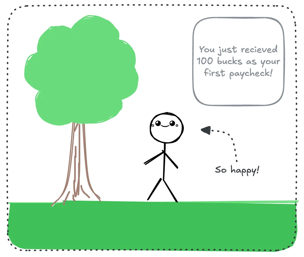
Let’s say you did some odd job for your neighbour and your naive lil self just got your first paycheck!
Now as you are walking down the street, you find this amazing place called a “Casino” and they tell you that you can double your money here. So you walk in…
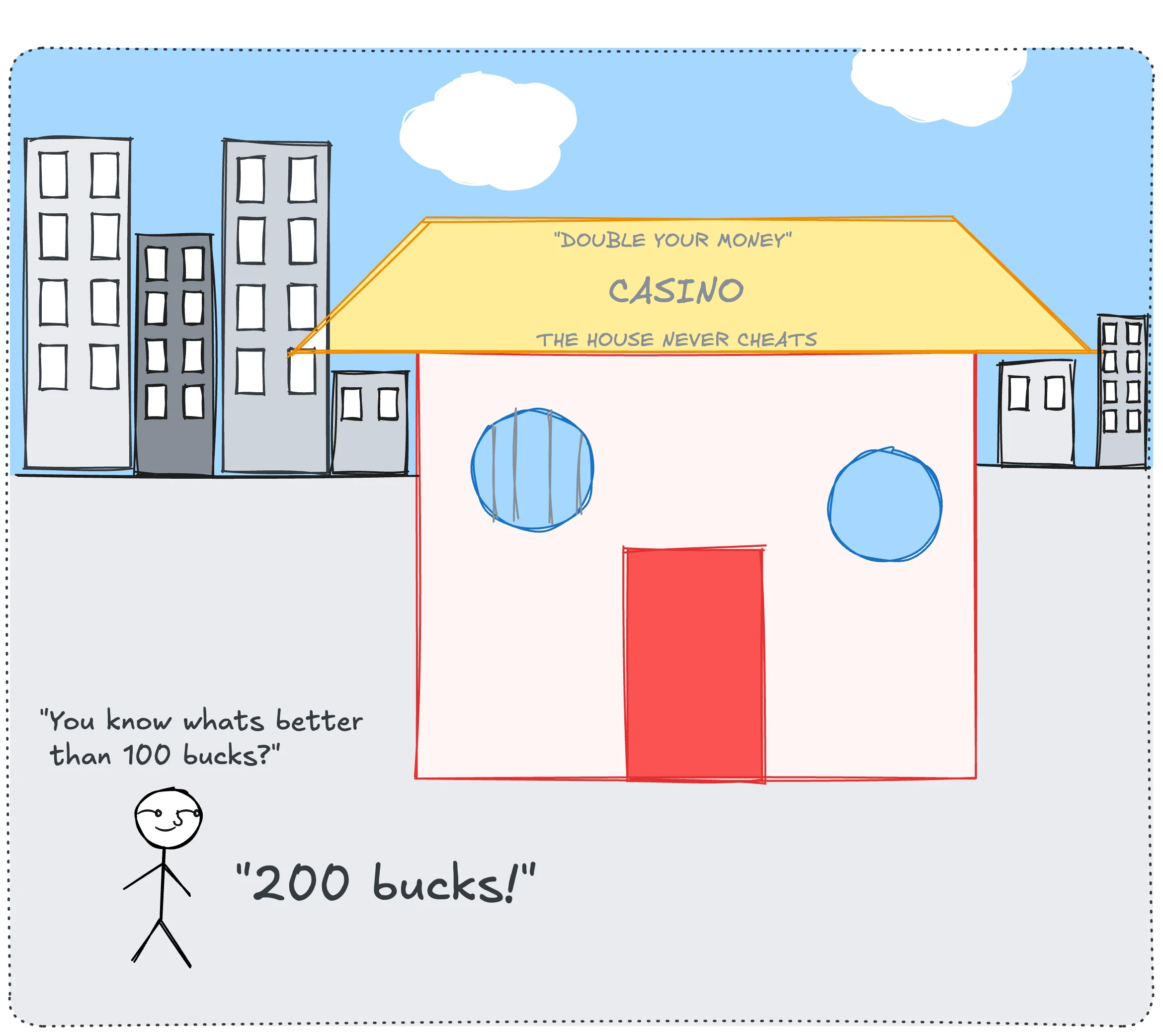
Oh god, what is this ungodly place! You are startled by all the bright lights, the money flying around, the vomit-colored carpet. But you are filled with joy, because you are about to double your money!!!

As you are walking through this labyrinth, you discover a fairly simple-looking machine. Well, a bunch of them in fact, lined up one after the other. They are slot machines!
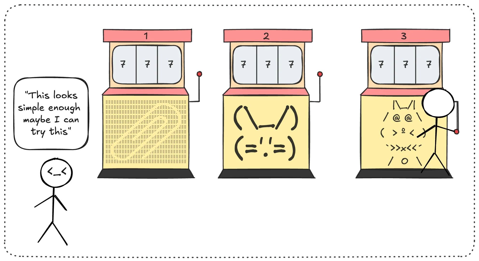
You think maybe you should try your luck here, as they seem simpler than poker: you just need to put money in, and get money out.
You try the first machine (let’s assume we put in a dollar and if we win we get an unspecified amount of money back; if we lose, THE MACHINE EATS OUR MONEY!!!). After 30 tries you find that instead of having more money, you have lost a significant amount.
This cannot be right, the hoarding said that the house never cheats (oh you naive kid, if only the world was as innocent as you are), and that you will in fact double your money. Sure, you will lose some tries, but if the claim is true, then on average, if you play enough times, you should win more than you lose!
So you start thinking and looking around, and that’s when you observe that the man on machine number 3 seems to be winning quite a fair bit. So you wait for him to leave, and once he does, you go to that machine and try it 30 times. Lo and behold… you have made more money than you started with! That’s when you realise… “THE HOUSE DOES IN FACT CHEAT!” (Who would have guessed, right?) Now, you are an intrepid person, who decides to fight back against this indignity with math and statistics.
So you formulate how you can win more money.
Let us assume we have $N$ tries (the amount of money), and we have $k$ options in front of us (the number of slot machines). We can assume that each of these $k$ options has an expected return, i.e. a mean around which there is some variance, but if played enough times, the average of what it gives back will converge to its true value. (This is the Law of Large Numbers: given enough tries, the black box will give its average output.)
So let’s assume this perfect, actual value of a slot machine $a$ can be represented as $q_\ast(a)$. But the problem is, any time we use it, it does not return the perfect $q_\ast(a)$ (because if it did, everyone would play all the slot machines once, figure out which gives the highest payout and just use that!). So instead we keep a running estimate $Q_n(a)$, which is the average of the rewards we have received from that machine so far.
We can write the true value as
\[q_*(a) \doteq \mathbb{E}[R_t \mid A_t = a]\]i.e. the expected reward $R_t$ given that we took the action $A_t = a$ (here an action is you choosing a particular slot machine).
If this is your first time seeing $\mathbb{E}[X]$, it essentially is the weighted mean of a distribution. In simpler terms it can be written as
\[\mathbb{E}[X] = \sum_i x_i \, p(x_i)\]i.e. the value of any given $x$ multiplied by the probability of that $x$ appearing, all added up. (Now if it is a uniform distribution, the probability of any given value occurring is $\frac{1}{\text{number of values}}$, so for something like the expected value of a die it would be
\[\mathbb{E}[\text{die}] = 1 \cdot \tfrac{1}{6} + 2 \cdot \tfrac{1}{6} + 3 \cdot \tfrac{1}{6} + 4 \cdot \tfrac{1}{6} + 5 \cdot \tfrac{1}{6} + 6 \cdot \tfrac{1}{6} = \frac{21}{6} = 3.5\]Notice that you can never actually roll a $3.5$! The expected value is not “the most likely outcome”, it is the average you would get if you rolled the die a huge number of times, which is exactly the Law of Large Numbers from above.)
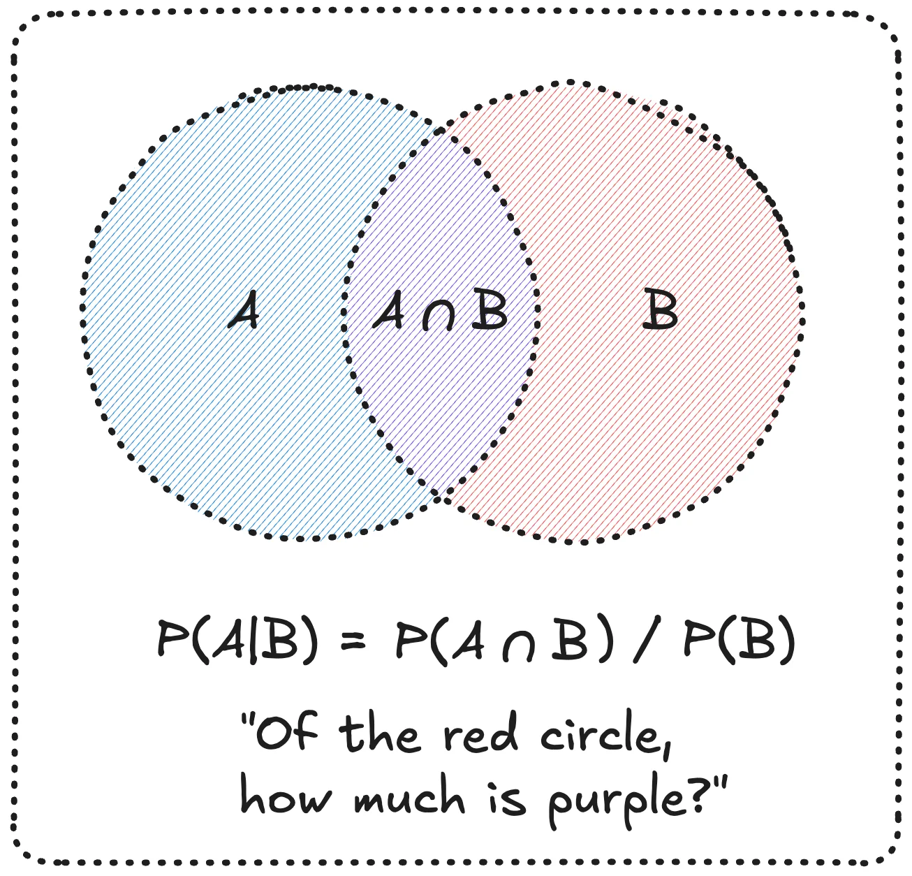
If this is your first time seeing the notation $\mathbb{E}[X \mid Y]$, it comes from conditional probability. $P(A \mid B)$ means: given that $B$ happened, what is the probability that $A$ also happened? I like to imagine this using Venn diagrams. Once we know $B$ happened, $B$ becomes our whole world, and we ask how much of that world is also $A$:
\[P(A \mid B) = \frac{P(A \cap B)}{P(B)}\]
The conditional expectation $\mathbb{E}[X \mid Y = y]$ uses this same idea, but instead of a probability it gives you an average: given that $y$ happened, what is the average value of $X$? It is just the weighted mean from above, with the conditional probabilities as the weights: $\mathbb{E}[X \mid Y = y] = \sum_x x \, P(X = x \mid Y = y)$. So $\mathbb{E}[R_t \mid A_t = a]$ reads “the average reward, given that we picked machine $a$”.
A further explanation of the above idea comes from introducing the ideas of posterior, prior, likelihood and marginal probability. While these sound like super complex words, they are quite simple to understand. We can write Bayes’ theorem as
\[P(A \mid B) = \frac{P(B \mid A)\, P(A)}{P(B)}\]Here $P(A \mid B)$ is the posterior, essentially the thing we are trying to find out (our belief about $A$ after seeing $B$). $P(A)$ is the prior, what we already believed about $A$ before seeing anything. $P(B \mid A)$ is the likelihood, how likely the evidence $B$ would be if $A$ were true. And $P(B)$ is called the marginal probability (or evidence), the overall probability of seeing $B$ at all.
We can write our estimate of a machine after it has been played $n-1$ times as
\[Q_n = \frac{R_1 + R_2 + \cdots + R_{n-1}}{n-1}\]This can be simplified (so that we do not need to store every single reward we have ever received). The estimate after $n$ rewards is
\[\begin{aligned} Q_{n+1} &= \frac{1}{n}\sum_{i=1}^{n} R_i \\ &= \frac{1}{n}\left(R_n + \sum_{i=1}^{n-1} R_i\right) \\ &= \frac{1}{n}\left(R_n + (n-1)\frac{1}{n-1}\sum_{i=1}^{n-1} R_i\right) \\ &= \frac{1}{n}\big(R_n + (n-1)Q_n\big) \\ &= \frac{1}{n}\big(R_n + nQ_n - Q_n\big) \\ &= Q_n + \frac{1}{n}\big[R_n - Q_n\big] \end{aligned}\]In the third line we multiplied and divided by $(n-1)$, which lets us spot that $\frac{1}{n-1}\sum_{i=1}^{n-1} R_i$ is just our old estimate $Q_n$. So now for each machine we only need to remember two numbers: the current estimate $Q_n$ and the count $n$.
This is a common trick in a lot of machine learning and you will see it in many papers. It is so common, in fact, that they often skip this exact derivation.
All in all, we can estimate the expected value of any slot machine simply by
\[\text{NewEstimate} \leftarrow \text{OldEstimate} + \text{StepSize}\big[\text{Reward} - \text{OldEstimate}\big]\]where the step size here is $\frac{1}{n}$.
You try this with the 3 machines, find the one which gave you the highest expected reward, make a huge buck and leave for home happy. You come back the next day, only to realise the casino caught on to what you were doing. So instead of 3 slot machines, they now have 10!!! machines.
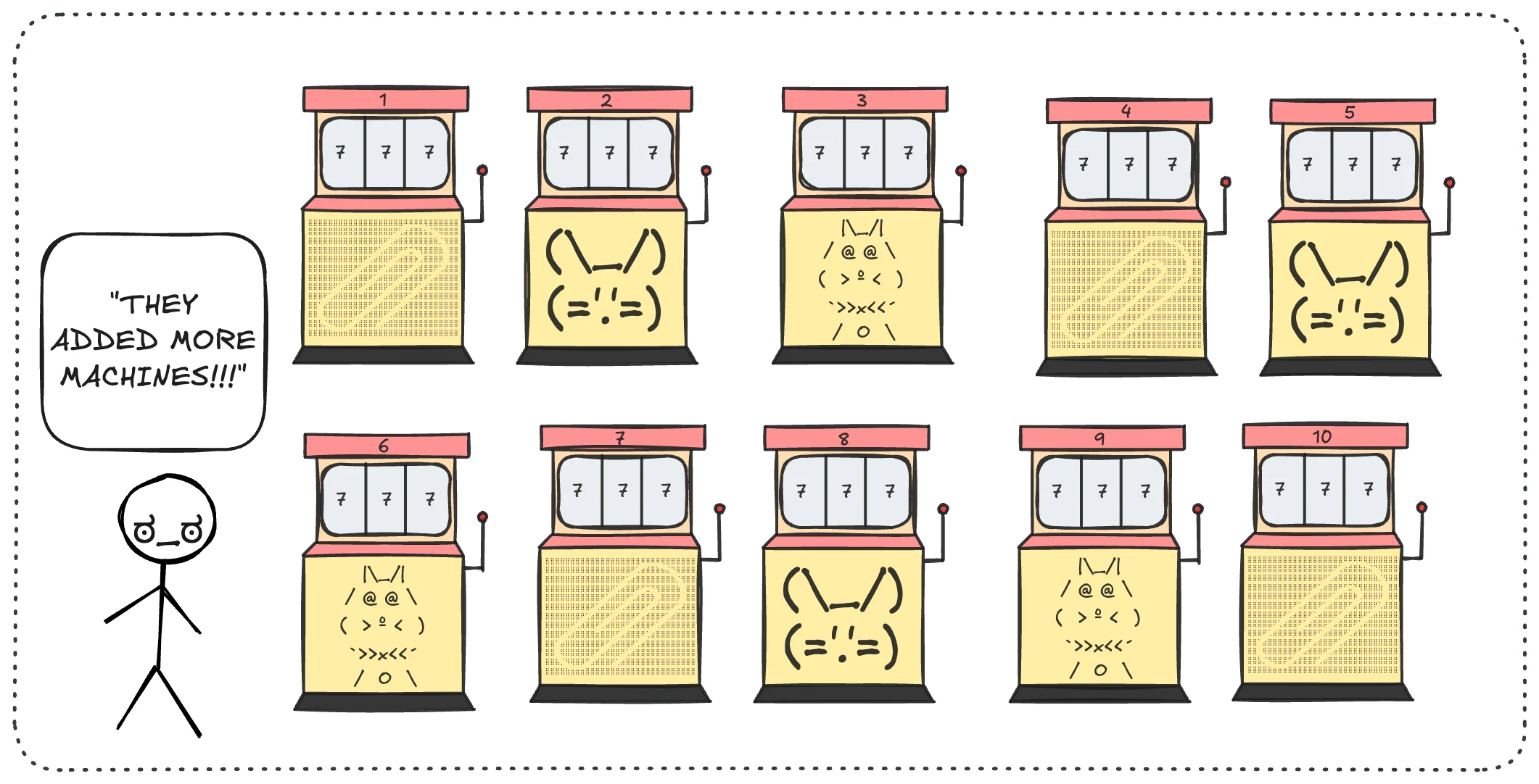
Your previous method will not work anymore, because you will waste a lot of tries just trying to find the optimal machine.
So you pull out your trusty notebook and start thinking:
“What if I assume that every machine gives on average 0 returns, then I try a machine and keep that estimate. Now that is my highest returning machine at the moment, so I will keep exploiting it, and at random times (let’s say $\varepsilon$ of the time) I will explore and try a random machine. If that gives me a greater reward than my current estimate for my current machine, I will stick to that!”
Wow, you mad genius. You write down your formula as such (mad geniuses need algorithms to work for some reason):
Note: This method is formally called $\varepsilon$-greedy action selection, and the dilemma here is between exploitation (just using the machine that has given you the highest average so far) and exploration (trying other machines which could potentially have a higher average). We vary the value of $\varepsilon$ to figure out what works best for us!
import numpy as np

rng = np.random.default_rng()

def bandit(q_true, action):
    # the slot machine: pays out a noisy reward around its (hidden) true value
    return rng.normal(loc=q_true[action], scale=1.0)

def epsilon_greedy(q_true, epsilon=0.1, steps=1000, initial_value=0.0):
    k = len(q_true)
    Q = np.full(k, initial_value)  # our estimate of each machine
    N = np.zeros(k)                # how many times we have played each machine
    rewards = np.zeros(steps)

    for t in range(steps):
        if rng.random() < epsilon:
            A = rng.integers(k)                           # explore
        else:
            A = rng.choice(np.flatnonzero(Q == Q.max()))  # exploit, breaking ties randomly
        R = bandit(q_true, A)
        N[A] += 1
        Q[A] += (1 / N[A]) * (R - Q[A])
        rewards[t] = R

    return Q, rewards

q_true = rng.normal(0, 1, size=10)  # 10 machines, each with a hidden true value
Q, rewards = epsilon_greedy(q_true, epsilon=0.1)
print("best machine:", q_true.argmax(), "| our best guess:", Q.argmax())
print("average reward:", rewards.mean())
Now now, I know it is tempting to skip reading the code above, but just give it a glance. It is quite simple and essential to our understanding.
You keep doing this for a while, but you are not getting the returns you would like, mostly because you are stuck exploiting only a few machines, while there are many more which could potentially have much higher rewards.
So you put on your thinking cap again.
“What if I assume every machine gives me, instead of 0, a value of 10 as the initial reward? This way I will be incentivized to try every machine at least once!”
And you have done it again! How do you even do it?
So now you modify your algorithm by changing $Q(a) \leftarrow 10$ (in the code above, that is just initial_value=10).
Formally this is called optimistic initial values, the idea is to force the agent to explore all options at least once! But it has a problem, as we will see soon…
You do this for a while, but again, you are distraught with the results. Because as you keep playing, you are also keeping track of how much money you are making and losing, and the graph does not look as good as you would like it to. The obvious answer seems to be that even after you try all the machines, in the end you still get stuck with a few machines, because you have no incentive to explore.
So you realise,
“What if I give these a high initial value, try them all, and also keep track of how many times I have tried each machine? This way, if I have been exploiting a specific machine for too long, I can look at which machines I have tried the least and play them. As these are the machines I have used the least, they have the highest chance of having a wrong $Q$ estimate.”
Oh my my my, are you Edward O. Thorp by any chance? You are on fire!!!
You modify how you pick your action $A_t$ as
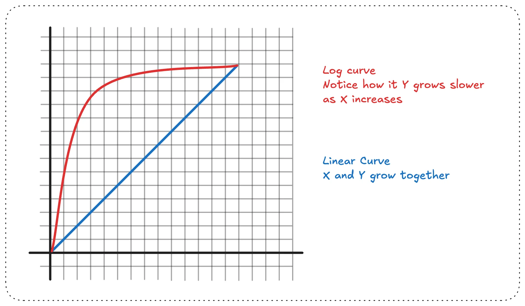
\[A_t \doteq \arg\max_a \left[ Q_t(a) + c\sqrt{\frac{\ln t}{N_t(a)}} \right]\]If the above equation feels like a big jump, let me simplify it. $\arg\max_a$ essentially means “pick the $a$ (the argument) that makes the thing in the brackets the biggest”. Here the thing in the brackets is our estimate plus an exploration bonus, so it is not just the highest expected return at that moment. $\ln$ is log with the natural base $e \approx 2.718$ (Euler’s number, read more about it here!). The way I like to remember log is something like the following. Imagine we take log with base 10, we can write $\log_{10}(1000) = 3$, i.e. how many times do we need to multiply 10 by itself to get 1000? Or, $10^x = 1000$. Obviously I took a very easy number because it shows the idea. The main reason we use log is because it scales the value much better: it keeps growing, but slower and slower. Compare the two graphs below for yourself to understand what I mean!
After 1000 pulls, $t$ is 1000 but $\ln t$ is only about 6.9. So the exploration bonus keeps nudging us to revisit neglected machines, but it never grows so fast that it drowns out what we have actually learned in $Q_t(a)$.
$N_t(a)$ is the number of times you have pulled the lever of a specific machine, $t$ is the total number of pulls so far (and $\ln t$ is its natural log, so the bonus grows slowly over time), and $c > 0$ controls how much you care about exploring. This will give a greater bonus to the machines you have tried the least, and a machine you have not tried at all ($N_t(a) = 0$) is treated as the best choice! (Now now, you are a smart person, think for a minute and realise this is simpler than it looks!)
NOTE: This is Upper Confidence Bound (UCB) action selection. The square-root term is the ‘uncertainty’ in the estimate. It shrinks as you play a machine more ($N_t(a)$ grows) and slowly grows for machines you ignore (because $\ln t$ keeps growing).
You employ this method, get an absurd amount of money and go home.
You come back the next day, again to milk these losers.
You start playing… and after a while you realise… the mean of all the machines keeps changing over time. YOU ARE SHOCKED!
“Are these guys changing the expected return of a machine over time?”
Guess what, the casino caught on to your tricks again, and they changed the machines overnight to have a moving expected mean.
You are in a dismal state, you have lost faith, time and money. You think of giving up. That is when you think of Papa John, and realise he would never have given up on making pizza to feed his family. So you… take out your notebook one more time, to teach this casino that you are better than them.
You look at your formula and realise the fatal flaw is in the step multiplier. With $\frac{1}{n}$, every new reward matters less and less as $n$ grows, which only makes sense if the values converge to one value. But now these values are never going to converge to one value. So you decide to replace that with a constant $\alpha$, so that recent rewards always count more than old ones!
\[Q_{n+1} = Q_n + \alpha\big[R_n - Q_n\big], \qquad \alpha \in (0, 1]\]This small change changes everything. Now you are back on track and winning some more!
Note: In RL terms, a problem where the true values keep changing over time is called a nonstationary problem. And the whole slot machine setup, where there is only one situation and you just keep picking an action, is called a non-associative problem, or the $k$-armed bandit problem.
The casino has had it with you and your math! The manager sends goons towards you to chase you out! You run towards the back exit…
…and just when you thought you had escaped your hell and were a free man, you realise… the back gate led to a maze, with only two ends: a dangerous fire pit, or the gates of Saintsbury (this is what we want!). Our hero is again in peril.
Just as you are about to lose hope, you spot something pinned on the wall by the entrance… A MAP of the maze! It shows every corridor, every dead end, where each turn leads, and where the fire pit and the gates of Saintsbury are. (How convenient… almost too convenient. But you are in no position to complain.)
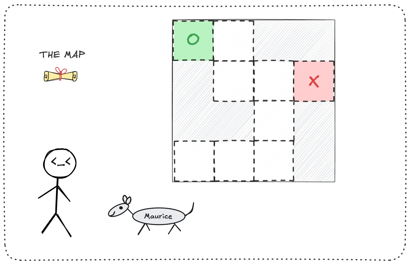
Our hero is quite exhausted from all the trouble and is in no position to solve this complex maze by hand. (The maze only looks simple to us as spectators, but in reality it is far too complex to be solved in mere seconds!)
That is when you take out your trusty sci-fi robo partner, Maurice! Now you must write an algorithm to run Maurice on, so Maurice can find the gates of Saintsbury for you and you can escape this maze!
Okay, now designing an algo for Maurice is going to be an arduous task, so you start by first breaking down your variables.
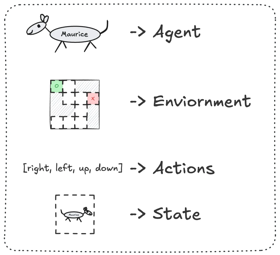
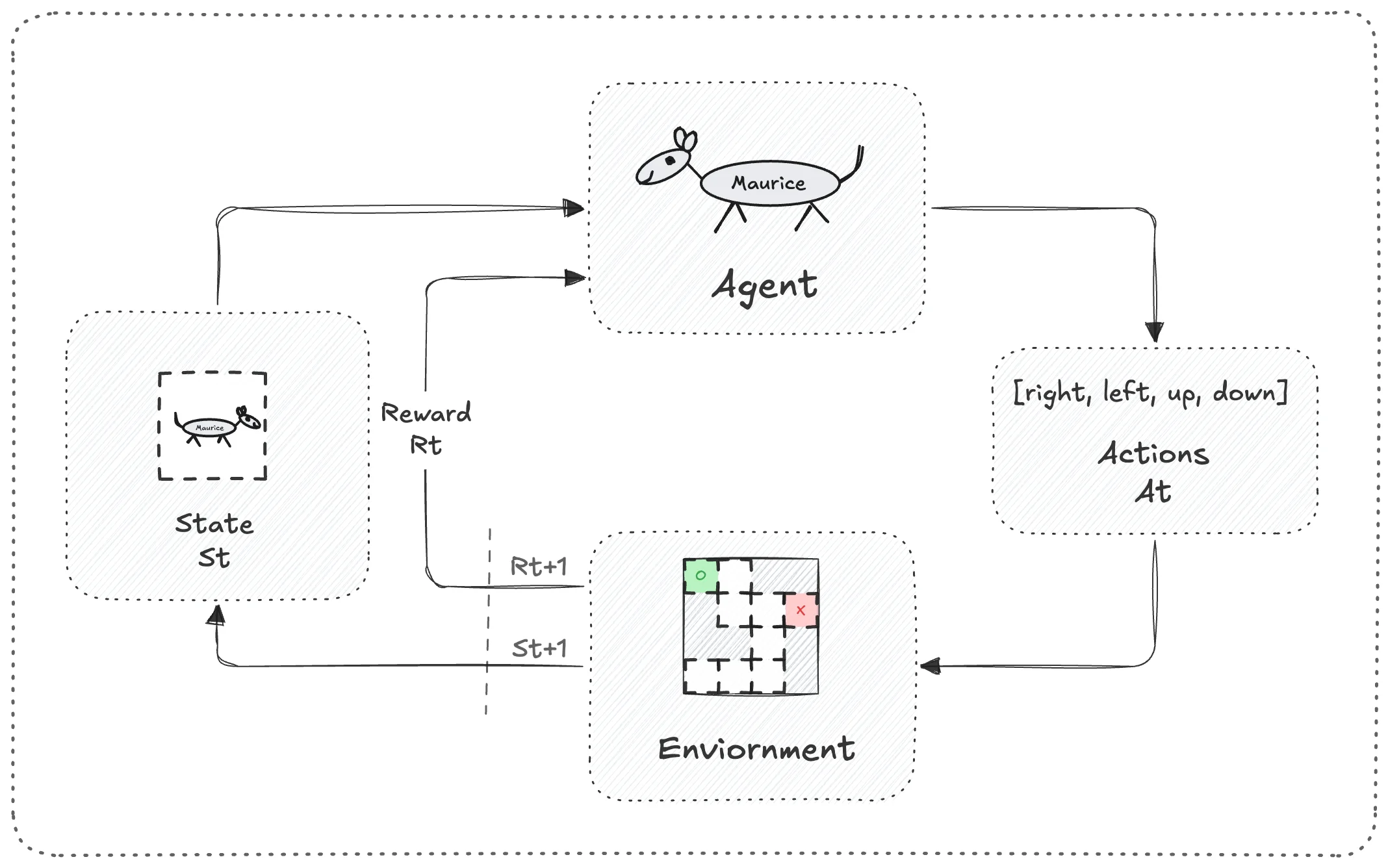
Maurice is your agent, who interacts with the environment, and where he is in the environment is his current state. Maurice can take actions (move up, down, left, right), and we would also like to give Maurice a reward if he gets the job done and saves us from this peril we are stuck in.
We can express the above idea in a simple diagram like below
[INSERT_IMAGE]
We can also rationalize that we start in a state $S_0$ (like standing at the entrance of the maze), take an action $A_0$ (like moving forward), and because of that get a reward $R_1$ (in this case the reward will be 0, because it is not like we got out!) and end up in state $S_1$ (the next tile). From $S_1$ we take action $A_1$, get a reward $R_2$, and so on… till we reach the end (the terminal state, in our case either impending doom in the fire pit or heaven by escaping through the gates of Saintsbury):
\[S_0, A_0, R_1, S_1, A_1, R_2, S_2, A_2, R_3, \dots\](Notice that the reward for the action taken at time $t$ is called $R_{t+1}$, because it arrives together with the next state $S_{t+1}$.)
The probability of ending up in state $s’$ with reward $r$, given that we were in state $s$ and took action $a$, can be written mathematically as
\[p(s', r \mid s, a) \doteq \Pr\{S_t = s', R_t = r \mid S_{t-1} = s, A_{t-1} = a\}\]Now now, this is nothing new, we already saw conditional probability in the beginning. This essentially says: given what is on the right is true (we are in a state and we took an action), what is the probability of the pair on the left (the state we will end up in and the reward we will get for it)!
And this is exactly what the map gives us! For every state and every action, we can read off where Maurice will end up and what reward he will get. (In a simple maze, each move takes you to exactly one next cell, so $p$ is just $1$ for that cell and $0$ for everything else. We write it as a probability so that it also works for trickier worlds, say a slippery floor that sometimes sends you somewhere else.)
Notice that $p$ only depends on where Maurice is now and what he does now, not on the whole path that got him there. This is called the Markov property, and a problem set up like this (states, actions, rewards and $p$) is called a Markov Decision Process (MDP).
Take this assumption for now, but later on we will expand more on MDPs, show how they work in most scenarios, and why they are the cornerstone of RL.
As you start formulating the problem, one of the first things that you realise is: the rewards are the easy part. Reaching the gates of Saintsbury gets $+1$, falling into the fire pit gets $-1$, and every other step gets $0$. But that is not enough! When Maurice is standing in some corridor in the middle of the maze, the reward there is $0$, which tells him nothing about whether he is one step from freedom or one step from the fire pit (the reason being… WE IN A MAZE! Every corridor looks the same!).
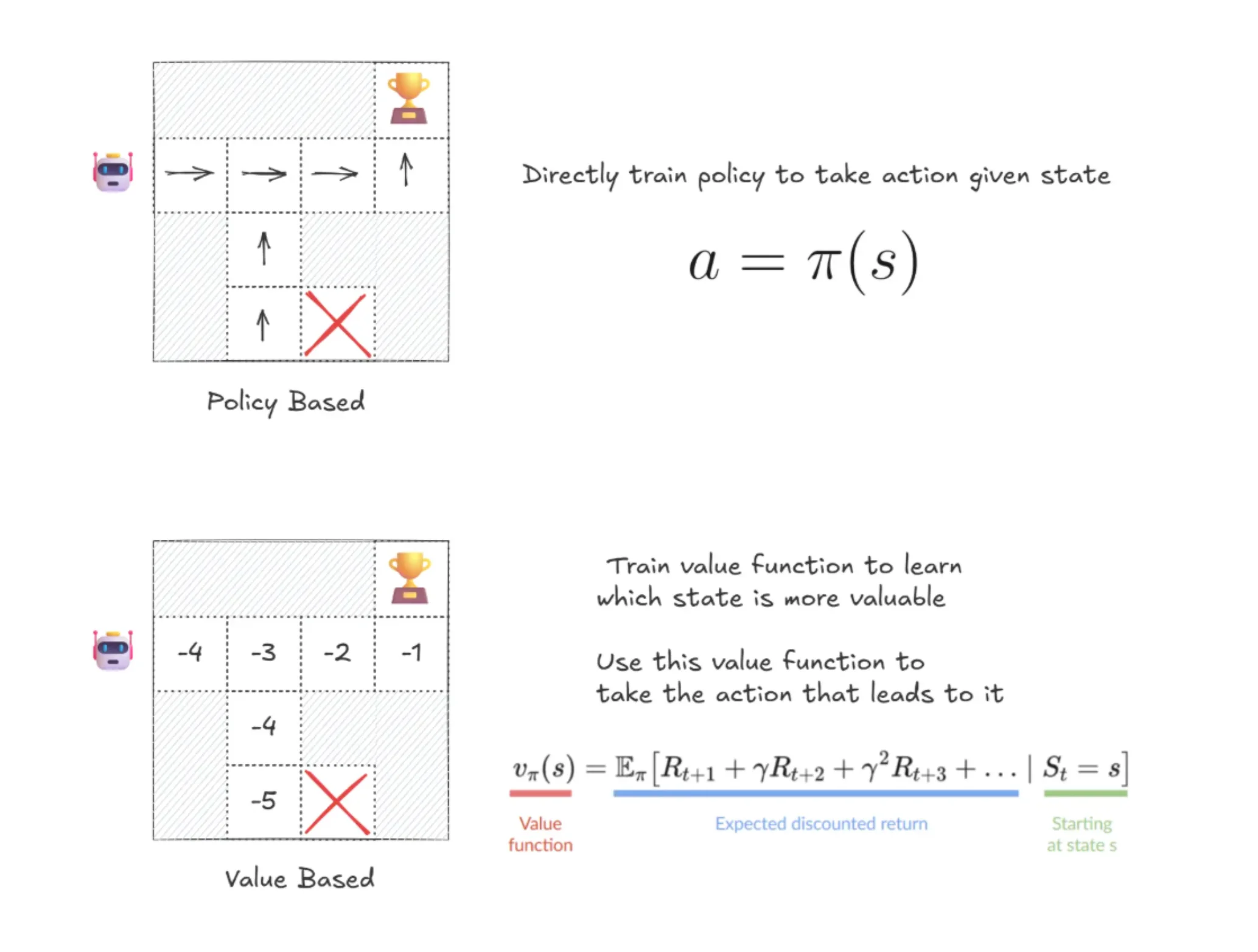
What Maurice needs is not the reward of each state, but how good each state is in the long run, i.e. how much reward he can expect to collect from there onwards. We call this the value of a state. Rewards are what the maze hands out, values are what Maurice has to figure out.
Let us slow down a bit if that felt like too much. Work backwards: if we get out, that gives us a reward. Our current problem is that we do not know how close we are to getting rewarded from any given state, so we need this idea of value. For instance, the value of the tile just before the gates is obviously higher than that of a tile 5 steps before it (once we add a little trick called discounting in a moment, which makes rewards that are further away count for less). And the value of the tile just before the fire pit is lower than that of the tiles which bring us closer to the gate.
The thing working in your favour is the map. Since we know the whole maze, Maurice does not need to take a single step to work these values out. He can sit right here and think. (Also I forgot to tell you, but he is essentially immortal, because you can respawn him every time he dies using your caller gadget, but let’s not test that.)
So you think, okay, maybe I can initialize a value for each state, then use the map to keep updating how close each state gets me to the end goal.
(Woah, that was a hard sentence to say, let’s break it down.)
Unlike the previous problem, where we got our reward immediately, here we get our reward after a while, so we can keep track of all the rewards within one run as
\[G_t \doteq R_{t+1} + R_{t+2} + R_{t+3} + \cdots + R_T\](the total reward you collect from time $t$ until the run ends at time $T$, by following whatever way of acting Maurice currently has. We call this the return, and we will talk about the optimal way of acting in a bit.)
But the problem with the above is that it can potentially explode (i.e. become numerically intractable, because the sum can get extremely large for large mazes, or even infinite if the task never ends). Another problem is that the agent will look far too much into the future, valuing every reward equally no matter how far away it is (this can lead Maurice to wander around collecting all the rewards, while what we want him to do is get us out ASAP). So what we can do is introduce an exponential weighting value $\gamma$ (with $0 \le \gamma \le 1$), called the discount factor:
\[G_t \doteq R_{t+1} + \gamma R_{t+2} + \gamma^2 R_{t+3} + \cdots = \sum_{k=0}^{\infty} \gamma^k R_{t+k+1}\]This is a good time to introduce a small idea called episodic and continuing tasks. The example we are dealing with now is episodic, i.e. it eventually ends. But there are multiple scenarios in real life where a task does not end. For instance, think of a thermostat trying to keep the temperature of a room constant. In all practicality it will never be done. Now you may wonder why we need to talk about the difference between episodic and continuing tasks. The big reason is that the math differs significantly between them. For instance, look at the above equation. It looks a lot like a geometric progression (read more here), and the sum of an infinite GP is very different from a finite one. In an episodic task the sum stops at $T$, so it is always finite. In a continuing task it never stops, and without $\gamma$ it could blow up to infinity. Interestingly, for $0 \le \gamma < 1$, $\sum_{k=0}^{\infty} \gamma^k = \frac{1}{1-\gamma}$, a constant. So if every reward is at most $R_{\max}$, the return can never be bigger than $\frac{R_{\max}}{1-\gamma}$, finite no matter how long the task runs! (And as a bonus, if you add the same constant $c$ to every reward, every state’s value just shifts by the same $\frac{c}{1-\gamma}$, so what really matters is the relative difference between rewards, not their actual values.) This part was more complex than I would have liked it to be, but as we move forward and do more RL, I will try to simplify it as we get more comfortable with this concept.
There is another benefit of $\gamma$ for the infinite case: it essentially makes the task pseudo-episodic from any state. For $n$ large enough, $\gamma^n$ will be very close to zero, so every reward after that point contributes almost nothing. (A handy rule of thumb: the agent effectively looks about $\frac{1}{1-\gamma}$ steps ahead, e.g. around 10 steps for $\gamma = 0.9$.)
This is our discounted return. Now, using this discounted return, we can determine how valuable any current state is as
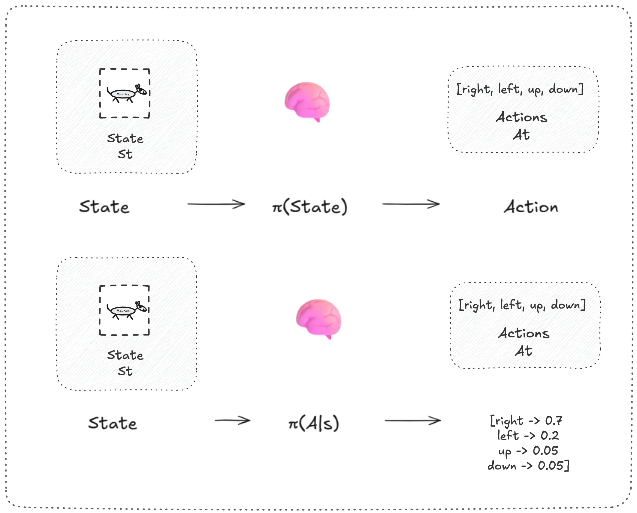
\[v_\pi(s) \doteq \mathbb{E}_\pi[G_t \mid S_t = s] = \mathbb{E}_\pi\left[\sum_{k=0}^{\infty} \gamma^k R_{t+k+1} \,\middle|\, S_t = s\right], \quad \text{for all } s \in \mathcal{S}\]Here $\pi$ is Maurice’s policy, i.e. his way of behaving: $\pi(a \mid s)$ is the probability that Maurice picks action $a$ when he is in state $s$. How valuable a state is depends on how Maurice behaves from there on, which is why $v$ carries that little $\pi$.
The above explanation makes sense logically, but let’s break it down mathematically as well. When we write $\mathbb{E}_\pi[X]$ we essentially “mean” (haha, pun intended) the expected value of the random variable $X$ when Maurice behaves according to $\pi$. (Quick short note: a random variable is an idea from probability and not the same thing as a variable in computer science. It is a quantity whose value depends on a random outcome, like the number a die lands on. Read more about it here.) Which we can break down as follows.
The return $G_t$ is a random variable: every time Maurice starts from $s$, he can end up taking a different path and collecting a different total reward. Which paths are likely depends on two things: Maurice’s choices ($\pi$) and how the maze responds ($p$). The little $\pi$ under the $\mathbb{E}$ is a reminder that the probabilities we average with come from following $\pi$. So using the weighted-mean definition from the beginning:
\[v_\pi(s) = \mathbb{E}_\pi[G_t \mid S_t = s] = \sum_{g} g \cdot \Pr_\pi(G_t = g \mid S_t = s)\]i.e. every possible return $g$, weighted by how likely Maurice is to get it when starting from $s$ and following $\pi$. A tiny example: say from tile $s$, Maurice goes left half of the time ($\pi(\text{left} \mid s) = 0.5$), which always ends up at the gates with a return of $+1$, and goes right the other half, which always ends in the fire pit with a return of $-1$. Then $v_\pi(s) = 0.5 \cdot (+1) + 0.5 \cdot (-1) = 0$. Change his policy to go left 90% of the time, and the same tile is now worth $0.9 - 0.1 = 0.8$. Same tile, same maze, different policy, different value. That is why $v$ needs its $\pi$!
Now the problem with the above formulation is that we cannot really work with it, so we have to break it down into what we understand.
We can break it down as the following
\[\begin{aligned} v_\pi(s) &\doteq \mathbb{E}_\pi[G_t \mid S_t = s] && (1) \\ &= \mathbb{E}_\pi[R_{t+1} + \gamma G_{t+1} \mid S_t = s] && (2) \\ &= \sum_a \pi(a \mid s) \sum_{s'} \sum_r p(s', r \mid s, a) \Big[ r + \gamma\, \mathbb{E}_\pi[G_{t+1} \mid S_{t+1} = s'] \Big] && (3) \\ &= \sum_a \pi(a \mid s) \sum_{s', r} p(s', r \mid s, a) \big[ r + \gamma\, v_\pi(s') \big], \quad \text{for all } s \in \mathcal{S} && (4) \end{aligned}\]Let’s go through it step by step.
(1) → (2). The return has a recursive structure. Pull the first reward out of the sum, and what is left is just the return from the next step, discounted once:
\[\begin{aligned} G_t &= R_{t+1} + \gamma R_{t+2} + \gamma^2 R_{t+3} + \cdots \\ &= R_{t+1} + \gamma\big(R_{t+2} + \gamma R_{t+3} + \cdots\big) \\ &= R_{t+1} + \gamma G_{t+1} \end{aligned}\][SELF-NOTE-SIMPLIFY-FROM-HERE]
So “everything from now on” = “the next reward” + $\gamma$ × “everything from the next step on”.
(2) → (3). The expectation is an average over everything random that happens in one step. Starting in state $s$, two random things happen:
- Maurice picks an action $a$, with probability $\pi(a \mid s)$ (his policy).
- The maze responds with a next state $s’$ and a reward $r$, with probability $p(s’, r \mid s, a)$.
So we average over both: we weight every possible $(a, s’, r)$ combination by its probability $\pi(a \mid s)\, p(s’, r \mid s, a)$, and for each one, what we get is the reward $r$ plus $\gamma$ times the expected return from wherever we landed, $\mathbb{E}\pi[G{t+1} \mid S_{t+1} = s’]$. (Why can we condition only on $s’$ and forget $s$ and $a$? The Markov property again: once you know where Maurice is now, how he got there does not change what happens next.)
If you want to see exactly how (3) falls out of (2), here it is slowly. We need just one tool, the law of total expectation: to find an average, you can split the world into cases, find the average within each case, and then take a weighted mean of those averages using how likely each case is:
\[\mathbb{E}[X \mid Y] = \sum_z P(Z = z \mid Y)\, \mathbb{E}[X \mid Y, Z = z]\](Example: the average height in a class = (fraction of girls × average height of girls) + (fraction of boys × average height of boys).)
The law of total expectation, slowly. Think of it as “an average of averages, weighted by how likely each case is”.
Let’s go back to the casino for a second. Say every evening you play machine A with probability $0.7$ and machine B with probability $0.3$. Machine A pays out $2$ on average and machine B pays out $10$ on average. What do you make on an average evening?
\[\mathbb{E}[\text{payout}] = \underbrace{0.7}_{P(\text{A})} \times \underbrace{2}_{\mathbb{E}[\text{payout} \mid \text{A}]} + \underbrace{0.3}_{P(\text{B})} \times \underbrace{10}_{\mathbb{E}[\text{payout} \mid \text{B}]} = 1.4 + 3 = 4.4\]Notice what we did not need: the full list of every possible payout and its probability. We only needed the average within each case, and how likely each case is. That is the whole trick.
Why is it true? Starting from the definition of expected value from the beginning, $\mathbb{E}[X] = \sum_x x \, P(X = x)$:
\[\begin{aligned} \mathbb{E}[X] &= \sum_x x \, P(X = x) && \text{(definition of expected value)} \\ &= \sum_x x \sum_z P(X = x, Z = z) && \text{(split } P(X = x) \text{ over every case } z\text{)} \\ &= \sum_x x \sum_z P(Z = z)\, P(X = x \mid Z = z) && \text{(conditional probability, rearranged)} \\ &= \sum_z P(Z = z) \sum_x x \, P(X = x \mid Z = z) && \text{(swap the order of the sums)} \\ &= \sum_z P(Z = z)\, \mathbb{E}[X \mid Z = z] && \text{(the inner sum is the average within case } z\text{)} \end{aligned}\]The third line is just the Venn diagram formula $P(A \mid B) = \frac{P(A \cap B)}{P(B)}$ multiplied out: $P(A \cap B) = P(B)\, P(A \mid B)$.
If we already know something, say $Y$ (for us, $S_t = s$), nothing changes. Every probability and expectation just gets a “$\mid Y$” attached, which gives the version written above.
One catch: the cases $z$ must cover every possibility, and no two of them can happen at the same time (machine A or machine B each evening, never both and never neither). Otherwise the weights don’t add up to 1 and the average comes out wrong.
In our maze, the “something we already know” is $S_t = s$, and we split twice:
- first on Maurice’s action: the cases are the actions $a$, weighted by $\pi(a \mid s)$,
- then on the maze’s response: the cases are the $(s’, r)$ pairs, weighted by $p(s’, r \mid s, a)$.
We apply it twice, first splitting on the action, then splitting on what the maze does:
\[\begin{aligned} &\mathbb{E}_\pi[R_{t+1} + \gamma G_{t+1} \mid S_t = s] && (2) \\ &= \sum_a \pi(a \mid s)\; \mathbb{E}_\pi[R_{t+1} + \gamma G_{t+1} \mid S_t = s, A_t = a] && (2a) \\ &= \sum_a \pi(a \mid s) \sum_{s'} \sum_r p(s', r \mid s, a)\; \mathbb{E}_\pi[R_{t+1} + \gamma G_{t+1} \mid S_t = s, A_t = a, S_{t+1} = s', R_{t+1} = r] && (2b) \\ &= \sum_a \pi(a \mid s) \sum_{s'} \sum_r p(s', r \mid s, a) \Big[ r + \gamma\, \mathbb{E}_\pi[G_{t+1} \mid S_t = s, A_t = a, S_{t+1} = s', R_{t+1} = r] \Big] && (2c) \\ &= \sum_a \pi(a \mid s) \sum_{s'} \sum_r p(s', r \mid s, a) \Big[ r + \gamma\, \mathbb{E}_\pi[G_{t+1} \mid S_{t+1} = s'] \Big] && (3) \end{aligned}\]- (2) → (2a): split on which action Maurice picks. The chance of each case is $\pi(a \mid s)$.
- (2a) → (2b): within each action, split again on where the maze sends him and what reward it gives. The chance of each case is $p(s’, r \mid s, a)$.
- (2b) → (2c): inside the expectation we now know $R_{t+1} = r$, so it is no longer random and comes out as just $r$ (the average of a known number is the number itself). The $\gamma$ also comes out, since the expectation of a constant times something is the constant times its expectation.
- (2c) → (3): the Markov property. The future return $G_{t+1}$ only depends on where Maurice is at $t+1$, so knowing $s$, $a$ and $r$ on top of $s’$ tells us nothing new, and we can drop them.
(3) → (4). Look at $\mathbb{E}\pi[G{t+1} \mid S_{t+1} = s’]$. It is “the expected return when starting from state $s’$ and following $\pi$”, which is exactly the definition of $v_\pi(s’)$! So we swap it in. (We also write $\sum_{s’}\sum_r$ as $\sum_{s’,r}$ to save some ink.)
And that is the magic: the value of a state is now written in terms of the immediate reward plus the discounted values of the states right after it. We no longer need to sum over the infinite future, we just look one step ahead.
This is popularly called the Bellman equation for $v_\pi$ (the state-value function).
[OPUS 5.5 NOTE: Skipped, and promised earlier (‘we will talk about the optimal way of acting in a bit’): (1) the action-value function $q_\pi(s,a)$, i.e. the value of taking action $a$ in $s$ and following $\pi$ afterwards; (2) the optimal value functions $v_\ast(s) = \max_\pi v_\pi(s)$ and $q_\ast(s,a)$; (3) the Bellman optimality equation, $v_\ast(s) = \max_a \sum_{s’,r} p(s’,r \mid s,a)[r + \gamma v_\ast(s’)]$. Value iteration below is literally this equation turned into an update, so introducing it here makes value iteration feel obvious instead of magic. Your Exercises 3.12, 3.13, 3.17, 3.25 and 3.26 already have all the pieces.]
We have the map and we have the Bellman equation, but we still need an algorithm to actually compute these values, right? How do we do that?
This family of methods, where you use a perfect model of the world (our map, i.e. $p$) to compute values by repeatedly applying the Bellman equation, is called Dynamic Programming (DP). Notice that Maurice never actually walks the maze here, all of it is done by thinking with the map. This is also called planning.
The first piece is what we call policy evaluation: given a policy $\pi$, compute $v_\pi$. The trick is to turn the Bellman equation into an update rule. Start with arbitrary guesses for $V(s)$, then sweep through all the states, replacing each $V(s)$ with the right-hand side of the Bellman equation computed using the current guesses. Keep sweeping until the values stop changing.
Iterative Policy Evaluation, for estimating V ≈ v_π

Input: π, the policy to be evaluated
Algorithm parameter: a small threshold θ > 0 determining accuracy of estimation
Initialize V(s) arbitrarily, for all s ∈ S, except that V(terminal) = 0

Loop:
    Δ ← 0
    Loop for each s ∈ S:
        v ← V(s)
        V(s) ← Σ_a π(a|s) Σ_{s',r} p(s',r|s,a) [r + γ V(s')]
        Δ ← max(Δ, |v − V(s)|)
until Δ < θ
This gives us the value of every state under the policy, but now we need to run Maurice on it, so he can find the values and follow them. “Following them” means that in every state, Maurice picks the action that leads to the best $r + \gamma V(s’)$ (this is called policy improvement). But once the policy changes, its values change too, so we evaluate again, improve again, and keep going until the policy stops changing. This is called policy iteration:
[OPUS 5.5 NOTE: The ‘policy improvement’ sentences above were added by me. Also skipped: the policy improvement theorem (§4.2), i.e. why acting greedily with respect to $v_\pi$ is guaranteed to give a policy at least as good as $\pi$. Without it, policy iteration looks like a heuristic rather than something guaranteed to reach the optimum.]
Policy Iteration (using iterative policy evaluation) for estimating π ≈ π*

1. Initialization
   V(s) ∈ ℝ and π(s) ∈ A(s) arbitrarily for all s ∈ S; V(terminal) = 0

2. Policy Evaluation
   Loop:
       Δ ← 0
       Loop for each s ∈ S:
           v ← V(s)
           V(s) ← Σ_{s',r} p(s',r|s,π(s)) [r + γ V(s')]
           Δ ← max(Δ, |v − V(s)|)
   until Δ < θ (a small positive number determining the accuracy of estimation)

3. Policy Improvement
   policy-stable ← true
   For each s ∈ S:
       old-action ← π(s)
       π(s) ← argmax_a Σ_{s',r} p(s',r|s,a) [r + γ V(s')]
       If old-action ≠ π(s), then policy-stable ← false
   If policy-stable, then stop and return V ≈ v* and π ≈ π*; else go to 2
We let Maurice go wild after telling him that he has to follow this algorithm.
But the problem that we realise is, Maurice is taking far too long! Because every round of policy evaluation sweeps through the whole maze again and again until the values have fully settled, and only then do we improve the policy a little. It would be much better if, in every sweep, Maurice directly used the value of the best action (the max) instead of waiting for the values of the current policy to settle. That way evaluation and improvement happen together in a single sweep. This is called value iteration and we can implement it as such!
[OPUS 5.5 NOTE: Optional, skipped: generalized policy iteration (§4.6), the big-picture idea that evaluation and improvement are two processes pulling against each other until they agree. Policy iteration, value iteration and almost every later RL algorithm are versions of it, so it is a strong closing idea for chapter 4. Asynchronous DP (§4.5) is fine to skip.]
Value Iteration, for estimating π ≈ π*

Algorithm parameter: a small threshold θ > 0 determining accuracy of estimation
Initialize V(s), for all s ∈ S⁺, arbitrarily except that V(terminal) = 0

Loop:
    Δ ← 0
    Loop for each s ∈ S:
        v ← V(s)
        V(s) ← max_a Σ_{s',r} p(s',r|s,a) [r + γ V(s')]
        Δ ← max(Δ, |v − V(s)|)
until Δ < θ

Output a deterministic policy, π ≈ π*, such that
    π(s) = argmax_a Σ_{s',r} p(s',r|s,a) [r + γ V(s')]
You stick this new algo inside of Maurice, he performs superbly and gets you the best path in only 5 iterations. Now you follow it, dancing and frog-leaping in happiness, because you have made so much money and have ESCAPED!!! with your freedom. As you reach near the gates of Saintsbury, you see a sight. A sight that shakes you, that mortifies you with fear!!
“Oh no, it is the manager!!!”
“No you fool, I am the manager’s brother. John!”
“Papa John???”
“What, no! Stop this malarkey. Anyhoo, if you wish to exit, you must answer this query of mine…”
” [INSERT_QUESTION] “
Wow, that is some question, quite perplexing if I say so myself. But our hero is left undaunted. You got this, let’s think it through, what do we know?
” ANSWER STEP BY STEP “
Our hero triumphs once again! You have been through numerous challenges, and you walk out of the gates of Saintsbury only to find out… it was all a ruse!!! No wonder the map was so conveniently placed there.
The manager is a mischievous man, he is playing with you. He is enjoying putting you through all this misery. But fret not, these little encumbrances will not shake your willpower.
This time we have no map, and the maze is as complex as it can be….
AND that’s all folks, join in for the next article to find out how our hero escapes this problem.
To add a bit of clarification if things went fast
Where to go from here
If you would like, I will recommend reading Reinforcement Learning: An Introduction by Sutton and Barto (it is free online!). You should have all the background needed to make sense of it now. If you do run into some issues and have trouble understanding, TELL ME, that will help me understand what exactly it was that I could not encapsulate.
Now, if I have helped you, even as a mere spectator, through an arduous journey filled with perils, laughs, cries and joy, then I have but one request: consider sharing this with your friends, so they can go on a very cool and fun journey as well!
Comments