
Evolution of LLMs
The landscape of language models(LMs) has evolved dramatically since the introduction of the Transformer architecture in 2017. Here we will explore the
- mathematical foundations
- architectural innovations
- training breakthroughs
We will talk about everything the code, math, and ideas that revolutionized NLP.
Additionally you can treat this blog as a sort of part 2, to my original blog on transformers which you can checkout here.
How this blog is structured
We will go year by year, going through the revolutionary ideas introduced by each paper.
In the beginning of each section, I have added the abstract, as well as the authors. I have done this to show you, the people were involved behind each idea. As well as what they felt like was the main contribution of their paper.
Below that I have provided the link to the original paper as well as my own implementation of it, subsequently there is a quick summary section which you can skim over if you feel like you know the crux behind the idea.
Note: All the quick summaries are AI generated, and may contain some mistakes. The core content is all human generated though, so it definitely contains mistakes :)
After that, each section contains intuition, code, and mathematical explanation (wherever required) for each idea. I have tried to add all the prerequisite knowledge wherever possible (Like the PPO section contains derivation of policy gradient methods, as well as explanation for TRPO). I have provided links to resources wherever I have felt I cannot provide enough background or do sufficient justice to the source material.
Additionally there has been a lot of innovation in vision modeling, TTS, Image gen, Video gen etc each of which deserves it’s own blog(And there will be!! I promise you that). As this is primarily an LLM blog, I will just give quick intro and links to some ground breaking innovations involving other ML papers.
Note: Do not take for granted all the hardware, data and benchmark innovations. Though I will briefly mention them. I implore you to explore them further if they interest you. This blog is strictly restricted to breakthroughs in Large Language Models, and mostly open source one’s. Even though current models by OpenAI, Anthropic, Google etc are amazing, not much is known about them to the public. So we will only briefly talk about them.
The AI timeline
This is a timeline of the most influential work. To read about more architectures that were huge at the time but died down eventually, consider going through the Transformer catalog.
The blog “Transformer models: an introduction and catalog — 2023 Edition” helped me immensely while making the timeline. Additionally this blog was helpful too.
| Links post 2019 are broken as it’s still work in progress |
2017
2018
- Universal Language Model Fine-tuning for Text Classification
- Deep contextualized word representations
- Improving Language Understanding by Generative Pre-Training
- SentencePiece: A simple and language independent subword tokenizer and detokenizer for Neural Text Processing
- BERT: Pre-training of Deep Bidirectional Transformers for Language Understanding
2019
- Language Models are Unsupervised Multitask Learners
- RoBERTa: A Robustly Optimized BERT Pretraining Approach
- DistilBERT, a distilled version of BERT: smaller,faster, cheaper and lighter
- BART: Denoising Sequence-to-Sequence Pre-training for Natural Language Generation, Translation, and Comprehension
- XLNet: Generalized Autoregressive Pretraining for Language Understanding
- Megatron-LM: Training Multi-Billion Parameter Language Models Using Model Parallelism
- Generating Long Sequences with Sparse Transformers
2020
- Reformer: The Efficient Transformer
- Longformer: The Long-Document Transformer
- GShard: Scaling Giant Models with Conditional Computation and Automatic Sharding
- Retrieval-Augmented Generation for Knowledge-Intensive NLP Tasks
- Big Bird: Transformers for Longer Sequences
- GPT-3
- Rethinking Attention with Performers
- T5
- Measuring Massive Multitask Language Understanding
- ZeRO (Zero Redundancy Optimizer)
- ELECTRA
- Switch Transformer
- Scaling Laws
2021
- RoFormer: Enhanced Transformer with Rotary Position Embedding
- Efficient Large-Scale Language Model Training on GPU Clusters Using Megatron-LM
- Transcending Scaling Laws with 0.1% Extra Compute
- Improving language models by retrieving from trillions of tokens
- CLIP
- Dall-e
- FSDP
- HumanEval
- LoRA
- Self-Instruct: Aligning Language Models with Self-Generated Instructions
- PaLM
- Gopher (DeepMind)
- Megatron-Turing NLG
2022
- EFFICIENTLY SCALING TRANSFORMER INFERENCE
- Fast Inference from Transformers via Speculative Decoding
- Chinchilla
- Chain-of-thought prompting
- InstructGPT
- BLOOM
- Emergent Abilities of Large Language Models
- Flash Attention
- Grouped-query attention
- ALiBi position encoding
- DeepSpeed Inference: Enabling Efficient Inference of Transformer Models at Unprecedented Scale
- Claude 1
- FLAN (Fine-tuned LAnguage Net) (Google)
- Red Teaming Language Models with Language Models
- HELM (Holistic Evaluation of Language Models)
- DALL-E 2 (OpenAI)
- Stable Diffusion (Stability AI)
- GPTQ
- Beyond the Imitation Game: Quantifying and extrapolating the capabilities of language models
- Minerva
- ChatGPT
2023
- Efficient Memory Management for Large Language Model Serving with PagedAttention
- QLoRA: Efficient Finetuning of Quantized LLMs
- Parameter-Efficient Fine-Tuning Methods for Pretrained Language Models: A Critical Review and Assessment
- FlashAttention-2: Faster Attention with Better Parallelism and Work Partitioning
- AWQ: Activation-aware Weight Quantization for LLM Compression and Acceleration
- Generative Agents: Interactive Simulacra of Human Behavior
- Voyager: An Open-Ended Embodied Agent with Large Language Models
- Universal and Transferable Adversarial Attacks on Aligned Language Models
- Tree of Thoughts: Deliberate Problem Solving with Large Language Models
- Mpt
- WizardLM: Empowering Large Language Models to Follow Complex Instructions
- DeepSpeed-Chat: Easy, Fast and Affordable RLHF Training of ChatGPT-like Models at All Scales
- GPT-4
- Mistral 7b
- LLaMA
- Mixtral 8x7B
- LLaMA 2
- Vicuna (LMSYS)
- Alpaca
- Direct Preference Optimization (DPO)
- Constitutional AI
- Toy Models of Superposition
- Towards Monosemanticity: Decomposing Language Models With Dictionary Learning
- PaLM 2
- LAION-5B (LAION)
- LIMA
- Mamba
- LLaVA (Visual Instruction Tuning)
- Claude 1/Claude 2
- Gemini
- Qwen
- Qwen-VL
- Phi-1
- Reinforced Self-Training (ReST) for Language Modeling
- The Era of 1-bit LLMs: All Large Language Models are in 1.58 Bits
2024
- Gemma
- Gemma 2
- Chatbot Arena: An Open Platform for Evaluating LLMs by Human Preference
- TinyLlama: An Open-Source Small Language Model
- MordernBert
- Jamba: A Hybrid Transformer-Mamba Language Model
- Claude 3
- LLaMA 3
- Gemini 1.5
- Qwen 2
- phi-2/phi-3
- OpenAI o1
- RSO (Reinforced Self-training with Online feedback)
- SPIN (Self-Played Improvement Narration)
- DBRX
- FlashAttention-3: Fast and Accurate Attention with Asynchrony and Low-precision
- Qwen 2.5 (Alibaba)
- DeepSeek 2.5 (DeepSeek)
- Claude 3.5 Sonnet (Anthropic)
- DeepSeek-R1 (DeepSeek)
- Phi 3
- Phi 4
- Self-Play Fine-Tuning Converts Weak Language Models to Strong Language Models
2025
Note: I am releasing this blog early as a preview to get feedback from the community. It is still a work in progress and I plan to explain as well as implement each paper from each year. Do let me know your thoughts through my socials, or in the comments below!!!
2017: The Foundation Year
Transformer
Link to paper: Attention is all you need
Link to implementation: [WORK IN PROGRESS]
Quick Summary
This is the famous “Attention Is All You Need” paper by Vaswani et al. that introduced the Transformer architecture - a groundbreaking neural network model that revolutionized natural language processing.
Key Innovation
The paper proposes replacing traditional recurrent neural networks (RNNs) and convolutional networks with a model based entirely on attention mechanisms. The core insight is that self-attention can capture dependencies between words regardless of their distance in a sequence, without needing to process them sequentially.
Architecture Highlights
- Encoder-Decoder Structure: 6 layers each, with multi-head self-attention and feed-forward networks
- Multi-Head Attention: Uses 8 parallel attention heads to capture different types of relationships
- Positional Encoding: Sine/cosine functions to inject sequence order information
- No Recurrence: Enables much better parallelization during training
Results The Transformer achieved state-of-the-art performance on machine translation tasks:
- 28.4 BLEU on English-to-German (WMT 2014)
- 41.8 BLEU on English-to-French
- Trained significantly faster than previous models (12 hours vs. days/weeks)
Impact This architecture became the foundation for modern language models like BERT, GPT, and others. The paper’s core principle - that attention mechanisms alone are sufficient for high-quality sequence modeling - fundamentally changed how we approach NLP tasks.
The work demonstrated superior performance while being more parallelizable and interpretable than previous sequence-to-sequence models.
THE foundational paper that introduced some key ideas such as:
- Scaled dot-product attention
- Multi-head attention mechanism
- Positional encodings
- Layer normalization
- Masked attention for autoregressive models
We have talked deeply about each of these topics previously and I implore you to check that part out here.
Problem
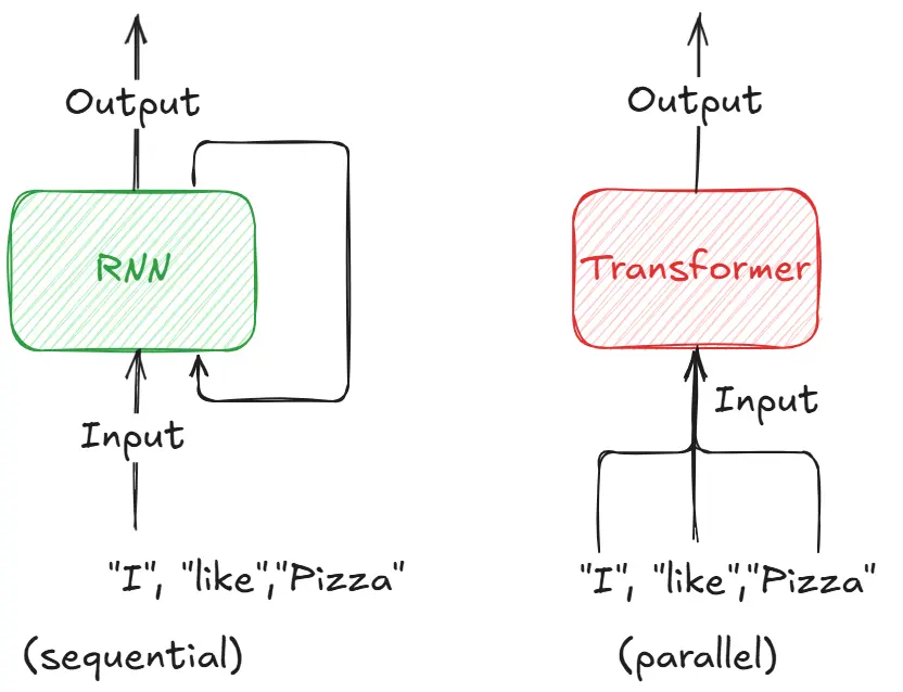
Sequential models like RNNs and LSTMs process text word-by-word, creating a fundamental bottleneck: each word must wait for the previous word to be processed. This sequential nature makes training painfully slow and prevents the model from understanding long-range dependencies effectively.
For example, in the sentence “The cat that lived in the house with the red door was hungry”, by the time the model reaches “was hungry”, it has largely forgotten about “The cat” due to the vanishing gradient problem. The model struggles to connect distant but related words.
Solution
The Transformer replaced sequential processing with parallel attention mechanisms. Instead of processing words one-by-one, it looks at all words simultaneously and uses attention to determine which words are most relevant to each other, regardless of their distance in the sentence.
This attention-based approach allows the model to directly connect “The cat” with “was hungry” in a single step, while also enabling massive parallelization during training - turning what used to take weeks into hours.
Training a Transformer
This is one topic that we didn’t talk about extensively so let’s go over it, because that is where the true beauty of GPT lies. How to train over huge amounts of data.
We will build iteratively, first starting small. And going massive as we approach the GPT paper.
This blog helped me with this section.
Preparing the data
The original Transformer was trained for neural machine translation using English-German sentence pairs. The data preparation involves several crucial steps:
# Data preparation
import torch
from torch.utils.data import DataLoader, Dataset
from torch.nn.utils.rnn import pad_sequence

def prepare_training_data(sentences):
    # 1. Add special tokens
    processed_sentences = []
    for sentence in sentences:
        processed_sentences.append("<START> " + sentence + " <EOS>")

    # 2. Create vocabulary
    vocab = build_vocab(processed_sentences)
    vocab_size = len(vocab)

    # 3. Convert to tensor sequences
    sequences = []
    for sentence in processed_sentences:
        tokens = sentence.split()
        sequence = torch.tensor([vocab[token] for token in tokens])
        sequences.append(sequence)

    # 4. Pad sequences
    padded_sequences = pad_sequence(sequences, batch_first=True, padding_value=0)

    return padded_sequences, vocab_size
-
Special tokens (
<START>and<EOS>): These tell the model where sentences begin and end. The<START>token signals the decoder to begin generation, while<EOS>teaches it when to stop. Without these, the model wouldn’t know sentence boundaries. As we will move through the years, we will see how the special tokens used in LLMs have evolved as well. For example, think what will happen inside an LLM when it encounters a token that it hasn’t seen during training, like a chinese character etc. -
Vocabulary creation: The vocabulary maps every unique word/token in the training data to a number. This is how we convert text (which computers can’t process) into numerical tensors (which they can). The vocabulary size determines the final layer dimension of our model.
-
Tensor conversion: Neural networks work with numbers, not words. Each word gets replaced by its vocabulary index, creating sequences of integers that can be fed into the model.
-
Padding: Sentences have different lengths, but neural networks need fixed-size inputs for batch processing. Padding with zeros makes all sequences the same length, enabling efficient parallel computation.
Key Training Innovations
The Transformer introduced several training techniques that became standard:
Teacher Forcing with Masking
# During training, decoder sees target sequence shifted by one position
encoder_input = source_sequence
decoder_input = target_sequence[:, :-1]  # Remove last token
decoder_output = target_sequence[:, 1:]  # Remove first token

# Look-ahead mask prevents seeing future tokens
def create_look_ahead_mask(seq_len):
    mask = torch.triu(torch.ones(seq_len, seq_len), diagonal=1)
    return mask.bool()

mask = create_look_ahead_mask(decoder_input.size(1))
Why this works: Teacher forcing trains the decoder to predict the next token given all previous tokens, without requiring separate training data. The input-output shift creates a “next token prediction” task from translation pairs. The look-ahead mask ensures the model can’t “cheat” by seeing future tokens during training - it must learn to predict based only on past context, just like during real inference.
Custom Learning Rate Schedule The paper introduced a specific learning rate scheduler that warms up then decays:
# Learning rate schedule from the paper
import math

class TransformerLRScheduler:
    def __init__(self, optimizer, d_model=512, warmup_steps=4000):
        self.optimizer = optimizer
        self.d_model = d_model
        self.warmup_steps = warmup_steps
        self.step_count = 0

    def step(self):
        self.step_count += 1
        lr = self.get_lr()
        for param_group in self.optimizer.param_groups:
            param_group['lr'] = lr

    def get_lr(self):
        arg1 = self.step_count ** -0.5
        arg2 = self.step_count * (self.warmup_steps ** -1.5)
        return (self.d_model ** -0.5) * min(arg1, arg2)
Why this schedule: The warmup phase gradually increases the learning rate, preventing the model from making drastic weight updates early in training when gradients are noisy. After warmup, the learning rate decays proportionally to the square root of the step number, allowing for fine-tuning as training progresses. This schedule was crucial for training stability with the Transformer’s deep architecture.
Padding Masks for Loss Computation
import torch.nn.functional as F

def masked_loss(target, prediction, pad_token=0):
    # Don't compute loss on padding tokens
    mask = (target != pad_token).float()

    # Reshape for cross entropy
    prediction = prediction.view(-1, prediction.size(-1))
    target = target.view(-1)
    mask = mask.view(-1)

    # Compute cross entropy loss
    loss = F.cross_entropy(prediction, target, reduction='none')
    masked_loss = loss * mask

    return masked_loss.sum() / mask.sum()
Why masking matters: Padding tokens (zeros) are artificial - they don’t represent real words. Computing loss on them would teach the model incorrect patterns and waste computational resources. The mask ensures we only compute loss on actual content, leading to more meaningful gradients and better learning. This also prevents the model from learning to predict padding tokens, which would be useless during inference.
Training Configuration
The original paper used these hyperparameters:
- Model size: 512 dimensions (base model)
- Attention heads: 8
- Encoder/Decoder layers: 6 each
- Feed-forward dimension: 2048
- Dropout: 0.1
- Optimizer: Adam with custom learning rate schedule
- Training time: ~12 hours on 8 P100 GPUs
The Training Loop
import torch
import torch.nn as nn
from torch.optim import Adam

def train_step(model, optimizer, scheduler, encoder_input, decoder_input, decoder_output):
    model.train()
    optimizer.zero_grad()

    # Forward pass
    prediction = model(encoder_input, decoder_input)

    # Compute masked loss and accuracy
    loss = masked_loss(decoder_output, prediction)
    accuracy = masked_accuracy(decoder_output, prediction)

    # Backward pass
    loss.backward()
    optimizer.step()
    scheduler.step()

    return loss.item(), accuracy.item()

# Main training loop
model = TransformerModel(src_vocab_size, tgt_vocab_size, d_model=512)
optimizer = Adam(model.parameters(), lr=1e-3, betas=(0.9, 0.98), eps=1e-9)
scheduler = TransformerLRScheduler(optimizer, d_model=512)

for epoch in range(num_epochs):
    for batch in dataloader:
        src_batch, tgt_batch = batch

        # Prepare inputs
        encoder_input = src_batch[:, 1:]     # Remove START token
        decoder_input = tgt_batch[:, :-1]    # Remove EOS token
        decoder_output = tgt_batch[:, 1:]    # Remove START token

        loss, accuracy = train_step(
            model, optimizer, scheduler,
            encoder_input, decoder_input, decoder_output
        )

        if step % 100 == 0:
            print(f'Epoch {epoch}, Step {step}, Loss: {loss:.4f}, Acc: {accuracy:.4f}')
Why This Training Approach Worked
- Parallelization: Unlike RNNs, all positions could be computed simultaneously
- Stable Gradients: Layer normalization and residual connections prevented vanishing gradients
- Efficient Attention: Scaled dot-product attention was computationally efficient
- Smart Masking: Prevented information leakage while enabling parallel training
This training methodology laid the groundwork for scaling to the massive language models we see today. The key insight was that with proper masking and attention mechanisms, you could train much larger models much faster than sequential architectures allowed.
While the original Transformer showed the power of attention-based training, it was still limited to translation tasks with paired data. The real revolution came when researchers realized they could use similar training techniques on massive amounts of unlabeled text data - setting the stage for GPT and the era of large language models.
RLHF - Reinforcement Learning from Human Preferences
Link to paper: Deep reinforcement learning from human preferences
Link to implementation: [WORK IN PROGRESS]
Quick Summary
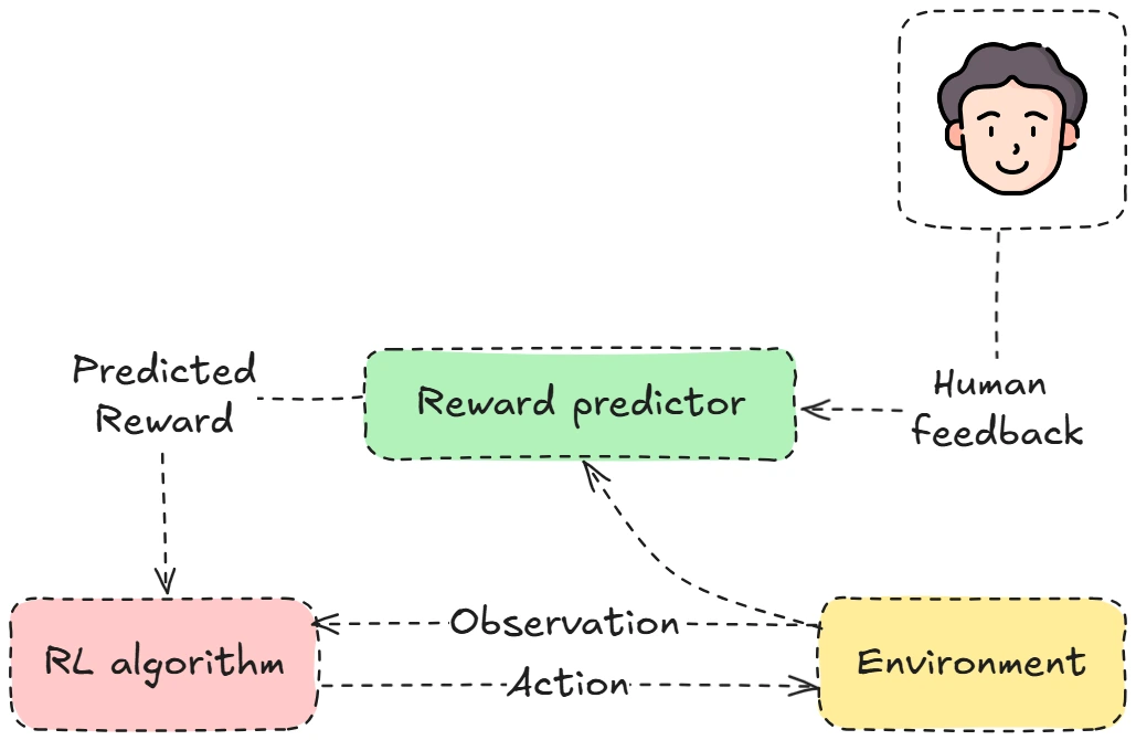
This paper presents a method for training reinforcement learning (RL) agents using human feedback instead of explicitly refined reward functions. Here’s a high-level overview:
The authors address a fundamental challenge in RL: for many complex tasks, designing appropriate reward functions is difficult or impossible. Instead of requiring engineers to craft these functions, they develop a system where:
- Humans compare short video clips of agent behavior (1-2 seconds)
- These comparisons train a reward predictor model
- The agent optimizes its policy using this learned reward function
Key contributions:
- They show this approach can solve complex RL tasks using feedback on less than 1% of the agent’s interactions
- This dramatically reduces the human oversight required, making it practical for state-of-the-art RL systems
- They demonstrate training novel behaviors with just about an hour of human time
- Their approach works across domains including Atari games and simulated robot locomotion
The technique represents a significant advance in aligning AI systems with human preferences, addressing concerns about misalignment between AI objectives and human values. By having humans evaluate agent behavior directly, the system learns rewards that better capture what humans actually want.
As mind boggling as it sounds, the famed algorithm RLHF came out in 2017, the same year attention is all you need came out. Let us understand the ideas put forth and why it was such a big deal.
(If you are not familiar with the idea of RL, I will recommend checking this small course by HuggingFace out)
Problem
Designing reward functions for complex behaviors is nearly impossible. How do you mathematically define “write a helpful response” or “be creative but truthful”? Traditional RL requires explicit numerical rewards for every action, but many desirable behaviors are subjective and context-dependent.
For example, it’s impossible to write code that scores joke quality, but humans can easily compare two jokes and say which is funnier.
Solution :
One possible solution is to allow a human to provide feedback on the agents’s current behavior and use this feedback to define the task. But this poses another problem, this would require hundreds of hours as well as domain experience. It was discovered by the researchers that preference modeling by a human even on a small subset provided great results.
An ideal solution will
- Enable us to solve tasks about which we can tell the desired behavior but not necessarily demonstrate or describe it.
- Allows systems to learn from non-expert users
- Scales to large problems
- Is economical
In their experiment, the researchers asked labellers to compare short video clips of the agent’s behavior. They found that by using a small sample of clips they were able to train the system to behave as desired.
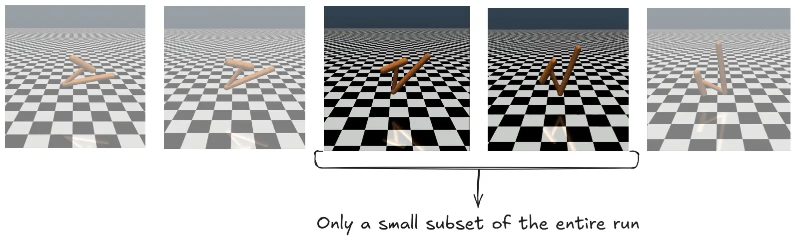 Image sourced from paper
The human observes the agent acting in the environment he then gives he’s feedback. Which is taken by reward predictor which numerical defines the reward. Which is sent to the RL algorithm this updates the agent based on the feedback and observation from the environment. That then changes the action of the agent.
This sounds simple enough in principle, but how do you teach a model to learn from these preferences. I.e reward modeling.
Note: We will be talking more in depth about RL algorithms in the next section. The topics in RL are rather complicated and usually talked in the end after an LLM is trained. So you can skip this part for now if it is daunting.
Reward predictor in RLHF
The following blogs helped me while writing this section
The reward predictor is trained to predict which of two given trajectories(σ¹, σ²) will be preferred by a human
Example:
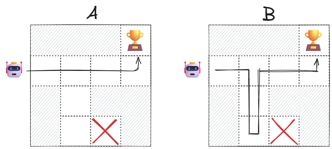
Imagine two robot trajectories:
- Trajectory A: Robot goes directly to the goal
- Trajectory B: Robot roams around then goes to the goal
A human would prefer A (more efficient). The reward model learns to assign higher values to the observation-action pairs in trajectory A, eventually learning that “efficient movement” correlates with human preference.
Reward predictor equation
\[\hat{P}\left[\sigma^{1} \succ \sigma^{2}\right]=\frac{\exp \sum \hat{r}\left(o_{t}^{1}, a_{t}^{1}\right)}{\exp \sum \hat{r}\left(o_{t}^{1}, a_{t}^{1}\right)+\exp \sum \hat{r}\left(o_{t}^{2}, a_{t}^{2}\right)}\]It is trained using cross-entropy loss to match human preferences:
\[\operatorname{loss}(\hat{r})=-\sum_{\left(\sigma^{1}, \sigma^{2}, \mu\right) \in D} \mu(1) \log \hat{P}\left[\sigma^{1} \succ \sigma^{2}\right]+\mu(2) \log \hat{P}\left[\sigma^{2} \succ \sigma^{1}\right]\]Mathematical Notation
- $\hat{P}\left[\sigma^{1} \succ \sigma^{2}\right]$: Predicted probability that trajectory segment $\sigma^{1}$ is preferred over trajectory segment $\sigma^{2}$
- $\hat{r}$: The learned reward function
- $o_{t}^{i}$: Observation at time $t$ in trajectory segment $i$
- $a_{t}^{i}$: Action at time $t$ in trajectory segment $i$
- $\sigma^{i}$: Trajectory segment $i$ (a sequence of observation-action pairs)
- $\exp$: Exponential function
- $\sum$: Summation over all timesteps in the trajectory segment
- $\operatorname{loss}(\hat{r})$: Cross-entropy loss function for the reward model
- $D$: Dataset of human preference comparisons
- $\mu$: Distribution over ${1,2}$ indicating human preference
- $\mu(1)$: Probability that human preferred segment 1
- $\mu(2)$: Probability that human preferred segment 2
- $\log$: Natural logarithm
Let us understand the Reward Function Fitting Process
The Preference-Predictor Model
The authors instead of directly creating a reward function (which rewards an agent when it does the desired behavior and punishes otherwise), they created a preference predictor. Which predicts which of the two given sequence of actions will be preferred by a human.
The Mathematical Formulation (Equation 1)
The equation P̂[σ¹ ≻ σ²] represents the predicted probability that a human would prefer trajectory segment σ¹ over segment σ².
Breaking down the formula:
- $\sigma^{[1]}$ and $\sigma^{[2]}$ are two different trajectory segments (short video clips of agent behavior)
- $o_{t}^{[i]}$ and $a_{t}^{[i]}$ represent the observation and action at time $t$ in trajectory $i$
- $\hat{r}(o_{t}^{[i]}, a_{t}^{[i]})$ is the estimated reward for that observation-action pair
- The formula uses the softmax function (exponential normalization):
This means:
- Sum up all the predicted rewards along trajectory 1
- Sum up all the predicted rewards along trajectory 2
- Apply exponential function to both sums
- The probability of preferring trajectory 1 is the ratio of exp(sum1) to the total exp(sum1) + exp(sum2)
The Loss Function
The goal is to find parameters for r̂ that make its predictions match the actual human preferences:
\[\operatorname{loss}(\hat{r}) = -\sum_{\left(\sigma^{[1]}, \sigma^{[2]}, \mu\right) \in D} \left[\mu([1])\log \hat{P}\left[\sigma^{[1]} \succ \sigma^{[2]}\right] + \mu([2])\log \hat{P}\left[\sigma^{[2]} \succ \sigma^{[1]}\right]\right]\]Where:
- $\left(\sigma^{[1]}, \sigma^{[2]}, \mu\right) \in D$ means we’re summing over all the comparison data in our dataset $D$
- $\mu$ is a distribution over ${1,2}$ indicating which segment the human preferred
- If the human strictly preferred segment 1, then $\mu([1]) = 1$ and $\mu([2]) = 0$
- If the human strictly preferred segment 2, then $\mu([1]) = 0$ and $\mu([2]) = 1$
- If the human found them equal, then $\mu([1]) = \mu([2]) = 0.5$
This is the standard cross-entropy loss function used in classification problems, measuring how well our predicted probabilities match the actual human judgments.
Consider reading this beautiful blog on Entropy by Christopher Olah, if you wish to gain a deeper understanding of cross-entropy.
The Bradley-Terry Model Connection
Note from Wikipedia: The Bradley–Terry model is a probability model for the outcome of pairwise comparisons between items, teams, or objects. Given a pair of items $i$ and $j$ drawn from some population, it estimates the probability that the pairwise comparison $i > j$ turns out true, as
\[\Pr(i>j) = \frac{p_i}{p_i + p_j}\]where $p_i$ is a positive real-valued score assigned to individual $i$. The comparison $i > j$ can be read as “i is preferred to j”, “i ranks higher than j”, or “i beats j”, depending on the application.
This approach is based on the Bradley-Terry model, which is a statistical model for paired comparisons. It’s similar to:
-
The Elo rating system in chess: Players have ratings, and the difference in ratings predicts the probability of one player beating another.
-
In this case: Trajectory segments have “ratings” (the sum of rewards), and the difference in ratings predicts the probability of a human preferring one segment over another.
In essence, the reward function learns to assign higher values to states and actions that humans tend to prefer, creating a preference scale that can be used to guide the agent’s behavior.
The most important breakthrough: We can align AI systems with human values using comparative feedback from non-experts. This insight would prove crucial when training language models - instead of trying to define “helpful” or “harmless” mathematically, we can simply ask humans to compare outputs.
This comparative approach scales much better than rating individual responses, making it practical for training large language models on human preferences.
| Fun story: One time researchers tried to RL a helicopter and it started flying backwards |
PPO: Proximal Policy Optimization

Link to paper: Proximal Policy Optimization Algorithms
Link to implementation: [WORK IN PROGRESS]
Quick Summary
This paper by John Schulman et al. from OpenAI introduces Proximal Policy Optimization (PPO), a family of policy gradient methods for reinforcement learning that achieves the reliability and data efficiency of Trust Region Policy Optimization (TRPO) while being much simpler to implement and more compatible with various neural network architectures.
Key contributions:
- A novel “clipped” surrogate objective function that provides a pessimistic estimate of policy performance
- An algorithm that alternates between data collection and multiple epochs of optimization on the same data
- Empirical validation showing PPO outperforms other online policy gradient methods across continuous control tasks and Atari games
- A balance between sample complexity, implementation simplicity, and computation time
The core innovation is their clipped probability ratio approach, which constrains policy updates without requiring the complex second-order optimization techniques used in TRPO. This makes PPO more practical while maintaining performance guarantees.
Another LLM algo that came out in 2017, and that too again by OpenAI. Really goes to show how much they tried to advance AI and be public about it (At least in the early days).
This is going to be math heavy so be prepared (Dw, I will guide you in each step)
Problem
However, there is room for improvement in developing a method that is scalable (to large models and parallel implementations), data efficient, and robust (i.e., successful on a variety of problems without hyperparameter tuning). Q-learning (with function approximation) fails on many simple problems and is poorly understood, vanilla policy gradient methods have poor data effiency and robustness; and trust region policy optimization (TRPO) is relatively complicated, and is not compatible with architectures that include noise (such as dropout) or parameter sharing (between the policy and value function, or with auxiliary tasks).
Essentially there were a lot of RL algorithms, but none of them worked efficiently at scale.
Solution
This paper seeks to improve the current state of affairs by introducing an algorithm that attains the data efficiency and reliable performance of TRPO, while using only first-order optimization. We propose a novel objective with clipped probability ratios, which forms a pessimistic estimate (i.e., lower bound) of the performance of the policy. To optimize policies, we alternate between sampling data from the policy and performing several epochs of optimization on the sampled data
The authors found a way to take the best RL algorithm of the time (TRPO) and make it work at scale.
The following blogs & articles helped me write this section
- Spinning up docs by OpenAI, consider going through this to help understand the nomenclature used throughout this section
- RL blogs by jonathan hui, they really simplified the ideas for me
- Understanding Policy Gradients, this blog really helped me understand the math behind the idea
- These blogs were extremely helpful too (each word is a different link)
- The bible of modern RL
What is Reinforcement Learning
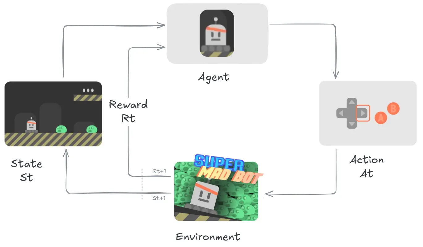 Image taken from HuggingFace Course
In RL we create an Agent (An ML model like Artificial Neural Network) give it a defined set of Actions $A_t$ (In this case it would be, move left, move right, Press A to shoot).
The agent then chooses an action and interacts with the Environment, which returns a new state as well as reward (positive if we survived or did a favourable outcome, negative if we die or do an unfavourable outcome).
Step by Step it looks something like this:
- The agent recieves state $S_0$ from the environment (In this that would be the first frame of the game)
- Based on state $S_0$, the agent takes action $A_0$ (chooses to move right)
- The environment goes to new frame, new state $S_1$.
- The environment gives the agent, reward $R_t$ (still alive!!!).
The idea behind RL is based on reward hypothesis, which states that
| All goals can be described as the maximization of the expected return (expected cumulative reward) |
Which can be mathematically represented as $R(\tau) = r_{t+1} + r_{t+2} + r_{t+3} + r_{t+4} + \ldots$ ($\tau$ read as tau)
Remember this, It will prove useful later.
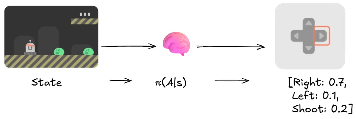
Policy π: The Agent’s Brain
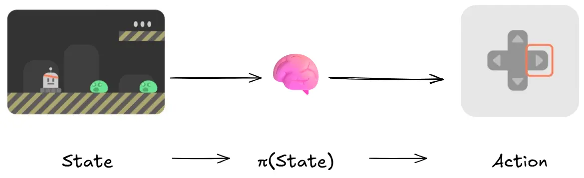
The Policy π is the brain of our Agent, it’s the function that tells an Agent what action it should take at a given state and time.
The policy is what we want to train and make an optimum policy π*, that maximizes expected return when the agent acts according to it. (remember that is the idea behind RL)
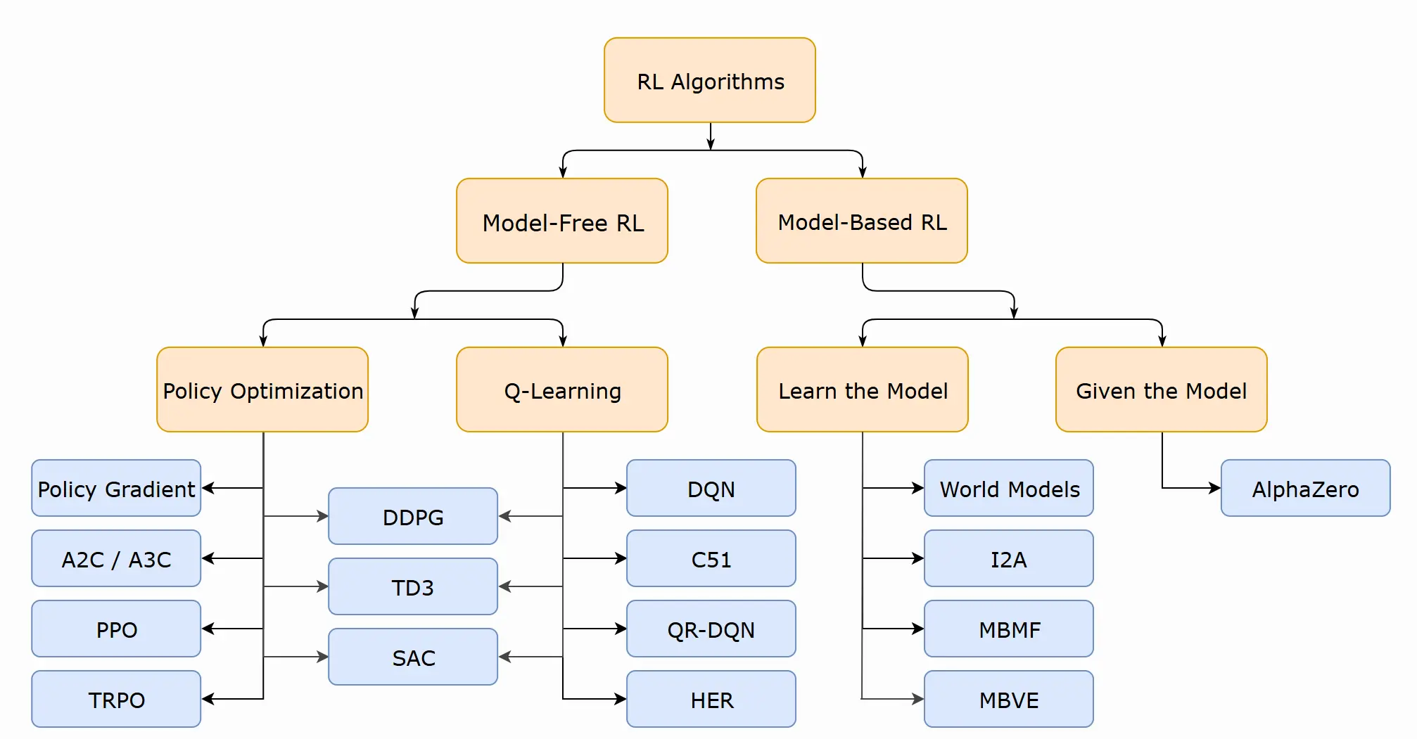 Image taken from OpenAI Spinning Up
There are many RL algorithms present that we can use to train the policy as you can see from the image above, But most of them are developed from two central methods:
- Policy based methods : Directly, by teaching the agent to learn which action to take, given the current state
- Value based methods : Indirectly, teach the agent to learn which state is more valuable and then take the action that leads to the more valuable states
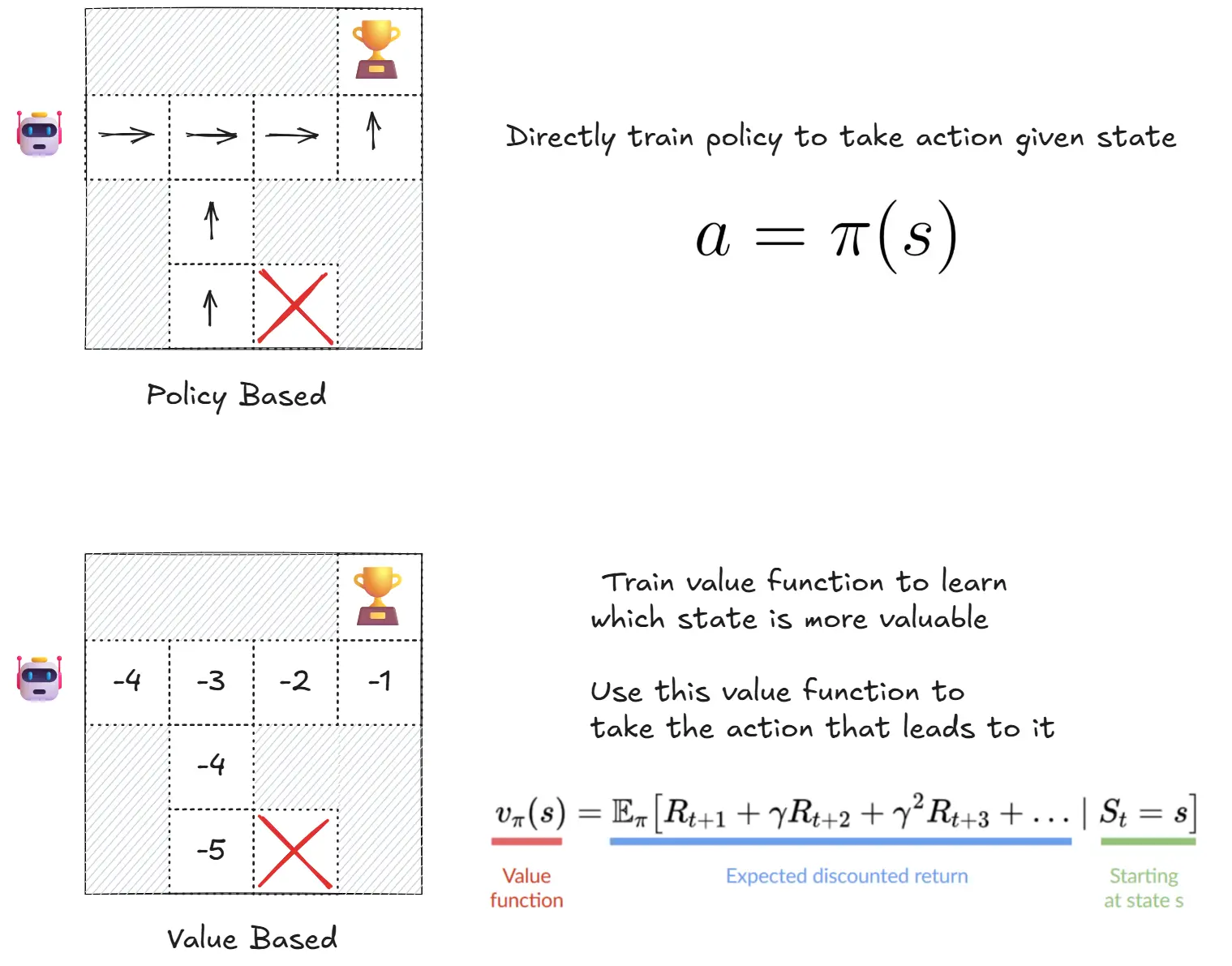 Image taken from HuggingFace Course
(Don’t get scared by the equations, I will explain them as we move forward. Also, this was a quick recap of RL, for a better deep dive. Consider going through the HF course)
As this section is dedicated to PPO, I will primarily be talking about the topics concerned with it. It can broadly be put in the following order:
- Policy Gradient Methods
- TRPO
- PPO
I am skipping over many other interesting and amazing algorithms like Q-Learning, DQN, Actor-critic etc. As they are not relevant to this section. I still implore you to explore them through the links I have provided to get a better, broader and deeper grasp of RL.
Before we move to the next section, I want to talk about a question that baffled me when I started learning about RL.
“Why do we need a value based approach”
Policy based approach seem to work great and are intuitive as well, given a state, choose an action. Then why do we use value based approaches. Needless complexity. Think for a minute then see the answer
Answer
Value-based methods shine in scenarios where policy-based methods struggle:
1. Discrete Action Spaces with Clear Optimal Actions In environments like Atari games or grid worlds, there’s often a single best action for each state. Value-based methods (like DQN) can directly learn which action has the highest expected return, making them sample-efficient for these deterministic scenarios.
2. Exploration Efficiency Value functions provide natural exploration strategies. Methods like ε-greedy or UCB can systematically explore based on value estimates. Policy methods often struggle with exploration, especially in sparse reward environments where random policy perturbations rarely discover good behavior.
3. Off-Policy Learning Value-based methods can learn from any data - even old experiences stored in replay buffers. This makes them incredibly sample-efficient. Policy methods traditionally required on-policy data, though modern techniques like importance sampling have bridged this gap.
4. Computational Efficiency In discrete action spaces, value-based methods often require just one forward pass to select an action (argmax over Q-values). Policy methods might need to sample from complex probability distributions or solve optimization problems.
Where Policy Methods Fail:
- High-dimensional discrete actions: Computing argmax becomes intractable
- Continuous control: You can’t enumerate all possible actions to find the maximum
- Stochastic optimal policies: Sometimes the best strategy is inherently random (like rock-paper-scissors), which value methods can’t represent directly
The truth is, both approaches are complementary tools for different types of problems.
Policy Gradient Methods
Policy gradient methods directly optimize a policy function by adjusting its parameters in the direction of greater expected rewards. They work by:
- Collecting experience (state-action pairs and rewards) using the current policy
- Estimating the policy gradient (the direction that would improve the policy)
- Updating the policy parameters using this gradient
The Gradient Estimator
In our discussion so far, we talked about deterministic policy based methods. Ie given a state, choose an action $\pi(s) = a$. But when we are talking about policy gradients, we use a stochastic policy based method. Ie given a state, return a probability distribution of actions $\pi(a|s) = P[A|s]$.
We also need to be aware of a few terms and mathematical tricks before moving forward:
-
Trajectory: A series of state action pair is called a trajectory.
\[\tau = (s_1,a_1,s_2,a_2,\ldots,s_H,a_H)\] -
Log derivative trick:
\[\nabla_\theta \log z = \frac{1}{z} \nabla_\theta z\]This trick allows us to convert the gradient of a probability into the gradient of its logarithm, which is computationally more stable and easier to work with.
(To derive it just apply chain rule and know that the derivative of $\log(x)$ = $1/x$)
-
Definition of Expectation:
For discrete distributions: \(\mathbb{E}_{x \sim p(x)}[f(x)] = \sum_x p(x)f(x) \tag{1}\)
For continuous distributions: \(\mathbb{E}_{x \sim p(x)}[f(x)] = \int_x p(x)f(x) \, dx \tag{2}\)
If you are new to the idea of expectation, Consider checking this amazing blog on the topic.
Deriving the Policy Gradient
Let $\tau$ be a trajectory (sequence of state-action pairs), $\theta$ be the weights of our neural network policy. Our policy $\pi_\theta$ outputs action probabilities that depend upon the current state and network weights.
We begin with the reward hypothesis: we want to maximize $R(\tau)$ where $\tau$ is a trajectory.
We can write the objective as the probability of a trajectory being chosen by the policy multiplied by the reward for that trajectory:
\[J(\theta) = \mathbb{E}_{\tau \sim \pi_\theta}[R(\tau)] = \sum_\tau \pi_\theta(\tau)R(\tau)\]This formulation is crucial because it connects:
- $\pi_\theta(\tau)$: How likely our current policy is to generate trajectory $\tau$
- $R(\tau)$: How much reward we get from that trajectory
For continuous trajectory spaces, we can write this as:
\[J(\theta) = \mathbb{E}_{\tau \sim \pi_\theta}[R(\tau)] = \int \pi_\theta(\tau)R(\tau)d\tau\]Now we can derive the policy gradient by taking the gradient of our objective:
\[\nabla_\theta J(\theta) = \nabla_\theta \int \pi_\theta(\tau)R(\tau)d\tau \tag{3}\] \[= \int \nabla_\theta \pi_\theta(\tau)R(\tau)d\tau \tag{4}\] \[= \int \pi_\theta(\tau) \frac{\nabla_\theta \pi_\theta(\tau)}{\pi_\theta(\tau)} R(\tau)d\tau \tag{5}\] \[= \int \pi_\theta(\tau) \nabla_\theta \log \pi_\theta(\tau) R(\tau)d\tau \tag{6}\] \[= \mathbb{E}_{\tau \sim \pi_\theta}[\nabla_\theta \log \pi_\theta(\tau) R(\tau)] \tag{7}\]Step-by-step explanation:
- (3) Start with gradient of our objective function
- (4) Push gradient inside the integral
- (5) Multiply and divide by $\pi_\theta(\tau)$
- (6) Apply the log derivative trick: $\nabla_\theta \log(z) = \frac{1}{z} \nabla_\theta z$
- (7) Convert back to expectation form
The trajectory probability factors as: \(\pi_\theta(\tau) = \prod_{t=0}^{T} \pi_\theta(a_t|s_t)\)
So the log probability becomes: \(\log \pi_\theta(\tau) = \sum_{t=0}^{T} \log \pi_\theta(a_t|s_t)\)
What does this mean for us? If you want to maximize your expected reward, you can use gradient ascent. The gradient of the expected reward has an elegant form - it’s simply the expectation of the trajectory return times the sum of log probabilities of actions taken in that trajectory.
In reinforcement learning, a trajectory $\tau = (s_1, a_1, s_2, a_2, \ldots, s_T, a_T)$ is generated through a sequential process. The probability of observing this specific trajectory under policy $\pi_\theta$ comes from the chain rule of probability.
| This is quite complex to intuitively understand in my opinion. Consider going through this stack exchange. Intuition: Let’s calculate the joint probability of a sequence like $P(\text{sunny weather, white shirt, ice cream})$ - what’s the chance it’s sunny outside, I’m wearing a white shirt, and I chose to eat ice cream all happening together? We can break this down step by step: First, what’s the probability it’s sunny outside? That’s $P(\text{sunny})$. Given that it’s sunny, what are the chances I wear a white shirt? That’s $P(\text{white shirt | sunny})$. Finally, given it’s sunny and I’m wearing white, what’s the probability I eat ice cream? That’s $P(\text{ice cream | sunny, white shirt})$. \(P(\text{sunny, white shirt, ice cream}) = P(\text{sunny}) \cdot P(\text{white shirt | sunny}) \cdot P(\text{ice cream | sunny, white shirt})\) By multiplying these conditional probabilities, we get the full joint probability. In reinforcement learning, trajectories work the same way: $P(s_1, a_1, s_2, a_2, \ldots)$ breaks down into “what state do we start in?” then “what action do we take?” then “where do we transition?” and so on. Each step depends only on what happened before, making complex trajectory probabilities manageable to compute and optimize. |
The joint probability of a sequence of events can be factored as: \(P(s_1, a_1, s_2, a_2, \ldots, s_T, a_T) = P(s_1) \cdot P(a_1|s_1) \cdot P(s_2|s_1, a_1) \cdot P(a_2|s_1, a_1, s_2) \cdots\)
However, in the Markov Decision Process (MDP) setting, we have two key assumptions:
- Markov Property: Next state depends only on current state and action: $P(s_{t+1}|s_1, a_1, \ldots, s_t, a_t) = P(s_{t+1}|s_t, a_t)$
- Policy Markov Property: Action depends only on current state: $P(a_t|s_1, a_1, \ldots, s_t) = \pi_\theta(a_t|s_t)$
| Chapter 3 of RL book by Sutton and Barto covers the topic well |
Applying these assumptions:
\[\pi_\theta(\tau) = \pi_\theta(s_1, a_1, \ldots, s_T, a_T) = p(s_1) \prod_{t=1}^{T} \pi_\theta(a_t|s_t)p(s_{t+1}|s_t, a_t)\] \[\underbrace{p(s_1) \prod_{t=1}^{T} \pi_\theta(a_t|s_t)p(s_{t+1}|s_t, a_t)}_{\pi_\theta(\tau)}\]- $p(s_1)$: Initial state distribution (environment dependent)
- $\pi_\theta(a_t|s_t)$: Policy probability of choosing action $a_t$ in state $s_t$
- $p(s_{t+1}|s_t, a_t)$: Environment transition probability (environment dependent)
When we take the log of a product, it becomes a sum:
\[\log \pi_\theta(\tau) = \log p(s_1) + \sum_{t=1}^{T} \log \pi_\theta(a_t|s_t) + \sum_{t=1}^{T} \log p(s_{t+1}|s_t, a_t)\]The first and last terms do not depend on $\theta$ and can be removed when taking gradients(and this is often done in practice):
- $\log p(s_1)$: Initial state is determined by environment, not our policy
- $\log p(s_{t+1}|s_t, a_t)$: Environment dynamics don’t depend on our policy parameters
Therefore: \(\nabla_\theta \log \pi_\theta(\tau) = \nabla_\theta \sum_{t=1}^{T} \log \pi_\theta(a_t|s_t) = \sum_{t=1}^{T} \nabla_\theta \log \pi_\theta(a_t|s_t)\)
So the policy gradient: \(\nabla_\theta J(\theta) = \mathbb{E}_{\tau \sim \pi_\theta}[\nabla_\theta \log \pi_\theta(\tau) R(\tau)]\)
becomes: \(\nabla_\theta J(\theta) = \mathbb{E}_{\tau \sim \pi_\theta}\left[\left(\sum_{t=1}^{T} \nabla_\theta \log \pi_\theta(a_t|s_t)\right) R(\tau)\right]\)
The trajectory return $R(\tau)$ is the total reward collected along the trajectory: \(R(\tau) = \sum_{t=1}^{T} r(s_t, a_t)\)
So our gradient becomes: \(\nabla_\theta J(\theta) = \mathbb{E}_{\tau \sim \pi_\theta}\left[\left(\sum_{t=1}^{T} \nabla_\theta \log \pi_\theta(a_t\|s_t)\right) \left(\sum_{t=1}^{T} r(s_t, a_t)\right)\right]\)
How do we compute expectations in practice?
We can’t compute the expectation $\mathbb{E}_{\tau \sim \pi{\theta}}[\cdot]$ analytically because:
- There are infinitely many possible trajectories
- We don’t know the environment dynamics $p(s_{t+1}|s_t, a_t)$
Instead, we use Monte Carlo sampling:
- Collect $N$ sample trajectories by running our current policy: ${\tau_1, \tau_2, \ldots, \tau_N}$
- Approximate the expectation using the sample average:
Applying Monte Carlo approximation
This is a fabulous video to understand Monte Carlo approximation.
Substituting our specific function: \(f(\tau) = \left(\sum_{t=1}^{T} \nabla_\theta \log \pi_\theta(a_t|s_t)\right) \left(\sum_{t=1}^{T} r(s_t, a_t)\right)\)
We get: \(\boxed{\nabla_\theta J(\theta) \approx \frac{1}{N} \sum_{i=1}^{N} \left(\sum_{t=1}^{T} \nabla_\theta \log \pi_\theta(a_{i,t}|s_{i,t})\right) \left(\sum_{t=1}^{T} r(s_{i,t}, a_{i,t})\right)}\)
\[\boxed{\theta \leftarrow \theta + \alpha \nabla_\theta J(\theta)}\]Where:
- $i$ indexes the sampled trajectories ($1$ to $N$)
- $t$ indexes time steps within each trajectory ($1$ to $T$)
- $(s_{i,t}, a_{i,t})$ is the state-action pair at time $t$ in trajectory $i$
The elegant result is that we only need gradients of our policy’s action probabilities - the environment dynamics completely disappear from our gradient computation! This makes policy gradients model-free and widely applicable.
And we use this policy gradient to update the policy $\theta$.
To get an intuition behind the idea consider reading the intuition part of this blog.
Policy Gradient for Continuous Space
So far, we’ve been working with discrete action spaces, like our super mad bot game where you can move left, move right, or press A to shoot. But what happens when your agent needs to control a robot arm, steer a car, or even select the “best” next token in language model fine-tuning? Welcome to the world of continuous control!
In discrete spaces, our policy outputs probabilities for each possible action:
- Move left: 30%
- Move right: 45%
- Shoot: 25%
But in continuous spaces, actions are real numbers. Imagine trying to control a robot arm where the joint angle can be any value between -180° and +180°. You can’t enumerate probabilities for every possible angle, there are infinitely many! (like in real numbers, you cannot even count the numbers present between 179 and 180… Where do you even begin?)
The solution is to make our neural network output parameters of a probability distribution (eg mean and standard deviation of a normal distribution) instead of individual action probabilities. Specifically, we use a Gaussian (normal) distribution.
Here’s how it works:
Instead of: $\pi_\theta(a_t|s_t) = \text{[probability for each discrete action]}$
We use: $\pi_\theta(a_t|s_t) = \mathcal{N}(f_{\text{neural network}}(s_t); \Sigma)$
Let’s break it down:
- Feed the state $s_t$ into your neural network
- Network outputs the mean $\mu = f_{\text{neural network}}(s_t)$ - this is the “preferred” action
- Choose a covariance matrix $\Sigma$ - this controls how much exploration/uncertainty around that mean
- Sample the actual action from the Gaussian: $a_t \sim \mathcal{N}(\mu, \Sigma)$
Now comes the amazing part. Remember our policy gradient formula?
\[\nabla_\theta J(\theta) = \mathbb{E}_{\tau \sim \pi_\theta}\left[\left(\sum_{t=1}^{T} \nabla_\theta \log \pi_\theta(a_t|s_t)\right) R(\tau)\right]\]The exact same formula still applies! We just need to compute $\nabla_\theta \log \pi_\theta(a_t|s_t)$ differently.
Let’s start with what a Multivariant Gaussian distribution actually looks like. For continuous actions, we assume they follow this probability density function:
\[f(x) = \frac{1}{(2\pi)^{d/2} |\Sigma|^{1/2}} \exp\left\{-\frac{1}{2}(x - \mu)^T \Sigma^{-1} (x - \mu)\right\}\]This looks scary, but it’s just the mathematical way of saying: “actions are most likely to be near the mean $\mu$, with spread determined by covariance $\Sigma$.”
(To understand where this idea comes from, read 13.7 from RL by Sutton and Barton)
Now, since our policy $\pi_\theta(a_t|s_t) = \mathcal{N}(f_{\text{neural network}}(s_t); \Sigma)$, we have:
\[\log \pi_\theta(a_t|s_t) = \log f(a_t)\]Taking the logarithm of our Gaussian:
\[\log \pi_\theta(a_t|s_t) = \log\left[\frac{1}{(2\pi)^{d/2} |\Sigma|^{1/2}} \exp\left\{-\frac{1}{2}(a_t - \mu)^T \Sigma^{-1} (a_t - \mu)\right\}\right]\]Using properties of logarithms ($\log(AB) = \log A + \log B$ and $\log(e^x) = x$):
\[\log \pi_\theta(a_t|s_t) = \log\left[\frac{1}{(2\pi)^{d/2} |\Sigma|^{1/2}}\right] - \frac{1}{2}(a_t - \mu)^T \Sigma^{-1} (a_t - \mu)\]The first term is just a constant (doesn’t depend on our neural network parameters $\theta$), so we can ignore it when taking gradients:
\[\log \pi_\theta(a_t|s_t) = -\frac{1}{2}(a_t - \mu)^T \Sigma^{-1} (a_t - \mu) + \text{const}\]Since $\mu = f_{\text{neural network}}(s_t)$, we can rewrite this as:
\[\log \pi_\theta(a_t|s_t) = -\frac{1}{2}||f(s_t) - a_t||^2_\Sigma + \text{const}\]Both the above equations are the same, it’s just a shorthand of writing it this way. It is also known as Mahalanobis distance squared.
Now we can compute the gradient with respect to our network parameters $\theta$:
\[\nabla_\theta \log \pi_\theta(a_t|s_t) = \nabla_\theta \left[-\frac{1}{2}(a_t - f(s_t))^T \Sigma^{-1} (a_t - f(s_t))\right]\]Let’s define $u = a_t - f(s_t)$ to simplify notation. Our expression becomes:
\[\nabla_\theta \log \pi_\theta(a_t|s_t) = \nabla_\theta \left[-\frac{1}{2} u^T \Sigma^{-1} u\right]\]Since $a_t$ and $\Sigma^{-1}$ don’t depend on $\theta$, we have:
\[\frac{\partial u}{\partial \theta} = \frac{\partial}{\partial \theta}(a_t - f(s_t)) = -\frac{\partial f(s_t)}{\partial \theta}\]For the quadratic form $u^T \Sigma^{-1} u$, using the chain rule:
\[\frac{\partial}{\partial \theta}(u^T \Sigma^{-1} u) = \frac{\partial u^T}{\partial \theta} \Sigma^{-1} u + u^T \Sigma^{-1} \frac{\partial u}{\partial \theta}\]Since $\Sigma^{-1}$ is symmetric, we can write:
\[\frac{\partial}{\partial \theta}(u^T \Sigma^{-1} u) = 2 u^T \Sigma^{-1} \frac{\partial u}{\partial \theta}\]Substituting back our expressions:
\[\nabla_\theta \log \pi_\theta(a_t|s_t) = -\frac{1}{2} \cdot 2 \cdot u^T \Sigma^{-1} \frac{\partial u}{\partial \theta}\] \[= -u^T \Sigma^{-1} \left(-\frac{\partial f(s_t)}{\partial \theta}\right)\] \[= u^T \Sigma^{-1} \frac{\partial f(s_t)}{\partial \theta}\]Substituting $u = a_t - f(s_t)$ back:
\[\nabla_\theta \log \pi_\theta(a_t|s_t) = (a_t - f(s_t))^T \Sigma^{-1} \frac{\partial f(s_t)}{\partial \theta}\]Since $\Sigma^{-1}$ is symmetric, $(a_t - f(s_t))^T \Sigma^{-1} = \Sigma^{-1}(a_t - f(s_t))$ when treated as a row vector, so we can write:
\[\nabla_\theta \log \pi_\theta(a_t|s_t) = \Sigma^{-1}(a_t - f(s_t)) \frac{\partial f(s_t)}{\partial \theta}\]Rearranging to match the original form:
\[\nabla_\theta \log \pi_\theta(a_t|s_t) = -\Sigma^{-1}(f(s_t) - a_t) \frac{\partial f(s_t)}{\partial \theta}\]This gradient has a beautiful intuitive interpretation:
- $(f(s_t) - a_t)$: The difference between what your network predicted and the action you actually took
- $\frac{df}{d\theta}$: How to change the network parameters to affect the output
- $\Sigma^{-1}$: Weighting factor (less weight for high-variance directions)
When you collect experience and compute rewards, here’s what happens:
- Good action taken ($R(\tau) > 0$): The gradient pushes $f(s_t)$ closer to the good action $a_t$
- Bad action taken ($R(\tau) < 0$): The gradient pushes $f(s_t)$ away from the bad action $a_t$
- Standard backpropagation: This gradient flows back through the network to update $\theta$
Our policy gradient update remains: \(\theta \leftarrow \theta + \alpha \nabla_\theta J(\theta)\)
The only difference is how we compute $\nabla_\theta \log \pi_\theta(a_t|s_t)$:
- Discrete case: Gradient of softmax probabilities
- Continuous case: Gradient of Gaussian log-likelihood (what we just derived!)
Everything else stays identical - collect trajectories, compute returns, update parameters. The same core algorithm seamlessly handles both discrete and continuous control problems!
Policy Gradient Improvements
There are two methods in which RL is trained
- Monte Carlo Learning: Cummulative reward of the entire episode (Entire run of the enviorment)
- Temporal Difference Learning: Reward is used to update policy in every step
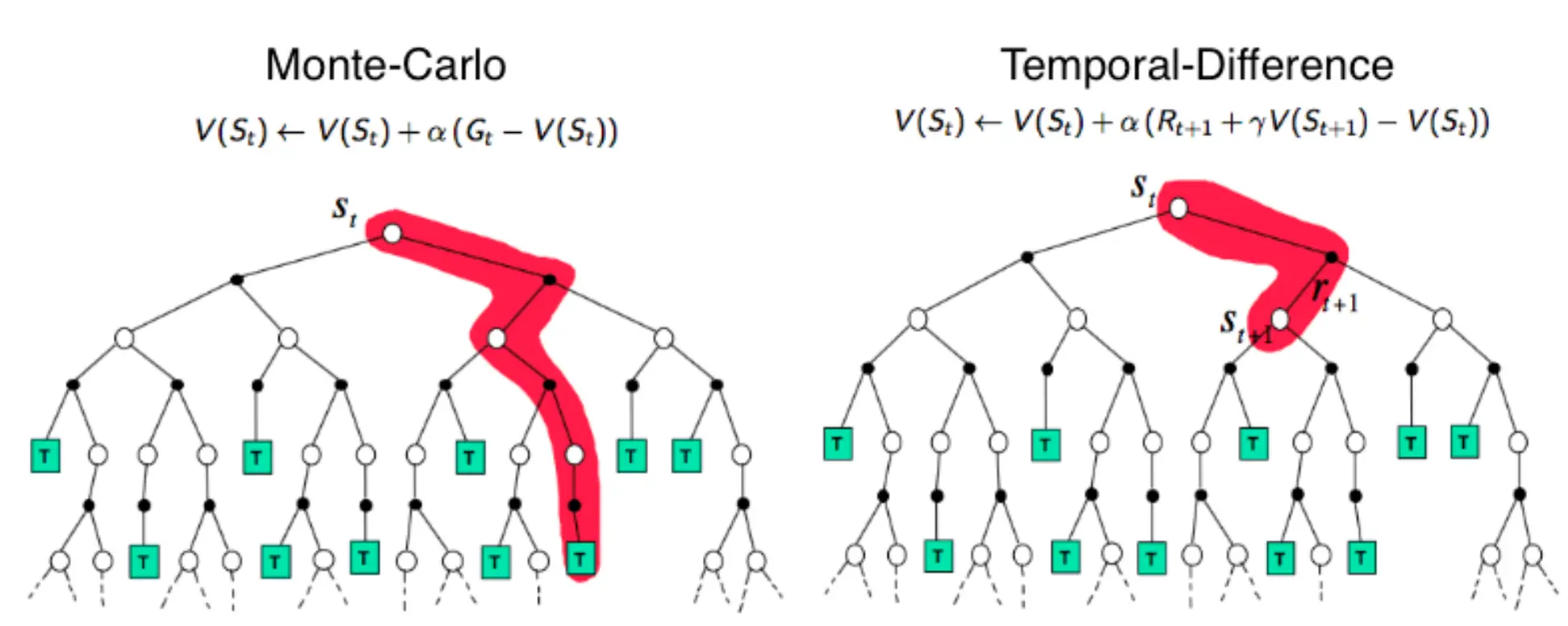 Image taken from Reinforcement Learning and Bandits for Speech and Language Processing: Tutorial, Review and Outlook
Policy Gradient (PG) uses MC this causes it to have low bias (Expected reward is close to actual reward, as the same policy is used throughout the run) but high variance (Some runs produce great results, some really bad).
| A stack exchange on bias & variance in RL |
Remember, our policy gradient formula is:
\[\nabla_\theta J(\theta) \approx \frac{1}{N} \sum_{i=1}^{N} \left(\sum_{t=1}^{T} \nabla_\theta \log \pi_\theta(a_{i,t}|s_{i,t})\right) \left(\sum_{t=1}^{T} r(s_{i,t}, a_{i,t})\right)\]We can rewrite this more compactly as:
\[\nabla_\theta J(\theta) \approx \frac{1}{N} \sum_{i=1}^{N} \sum_{t=1}^{T} \nabla_\theta \log \pi_\theta(a_{i,t}|s_{i,t}) \cdot Q(s_{i,t}, a_{i,t})\]Where $Q(s,a)$ represents the total reward we get from taking action $a$ in state $s$ (this is called the Q-function or action-value function).
The Baseline Trick
Here’s a mathematical insight: we can subtract any term from our gradient as long as that term doesn’t depend on our policy parameters $\theta$.
Why? Because: \(\nabla_\theta [f(\theta) - c] = \nabla_\theta f(\theta) - \nabla_\theta c = \nabla_\theta f(\theta) - 0 = \nabla_\theta f(\theta)\)
So instead of using $Q(s,a)$ directly, we can use $Q(s,a) - V(s)$, where $V(s)$ is some baseline function.
The most natural choice for baseline is $V(s) =$ the expected reward from state $s$ (The value function). This represents “how good is this state on average?”
Our new gradient becomes: \(\nabla_\theta J(\theta) \approx \frac{1}{N} \sum_{i=1}^{N} \sum_{t=1}^{T} \nabla_\theta \log \pi_\theta(a_{i,t}|s_{i,t}) \cdot (Q(s_{i,t}, a_{i,t}) - V(s_{i,t}))\)
This is defined as the Advantage Function: \(A^{\pi}(s,a) = Q^{\pi}(s,a) - V^{\pi}(s)\)
The advantage function answers the question: “How much better is taking action $a$ in state $s$ compared to the average action in that state?”
- $A(s,a) > 0$: Action $a$ is better than average → increase its probability
- $A(s,a) < 0$: Action $a$ is worse than average → decrease its probability
- $A(s,a) = 0$: Action $a$ is exactly average → no change needed
Our final policy gradient becomes: \(\boxed{\nabla_\theta J(\theta) \approx \frac{1}{N} \sum_{i=1}^{N} \sum_{t=1}^{T} \nabla_\theta \log \pi_\theta(a_{i,t}|s_{i,t}) \cdot A^{\pi}(s_{i,t}, a_{i,t})}\)
Let’s understand why this reduces variance with an example:
Situation 1: Trajectory A gets +10 rewards, Trajectory B gets -10 rewards
- If average performance is 0: $A_A = +10$, $A_B = -10$
- Result: Increase A’s probability, decrease B’s probability ✓
Situation 2: Trajectory A gets +10 rewards, Trajectory B gets +1 rewards
- If average performance is +5.5: $A_A = +4.5$, $A_B = -4.5$
- Result: Increase A’s probability, decrease B’s probability ✓
Even when both trajectories have positive rewards, the advantage function correctly identifies which one is relatively better!
In deep learning, we want input features to be zero-centered. The advantage function does exactly this for our rewards:
- Without baseline: All positive rewards → always increase probabilities
- With advantage: Rewards centered around zero → increase good actions, decrease bad ones
This gives our policy gradient much clearer, less conflicting signals, significantly reducing variance and improving convergence.
Vanilla Policy Gradient Algorithm
Now that we understand the advantage function, let’s see how it all comes together in the complete algorithm:
\[\nabla U(\theta) \approx \hat{g} = \frac{1}{m} \sum_{i=1}^{m} \nabla_\theta \log P(\tau^{(i)}; \theta)(R(\tau^{(i)}) - b)\](The notation may change from paper to paper, but the core idea remains the same)
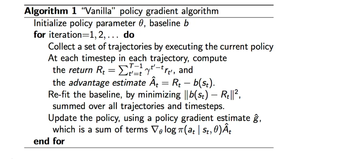 Image taken from RL — Policy Gradient Explained
Reward Discount
There’s one more important technique that further reduces variance: reward discounting.
Reward discount reduces variance by reducing the impact of distant actions. The intuition is that actions taken now should have more influence on immediate rewards than on rewards received far in the future.
You can think of it in terms of money, would rather have money right now, or have it later.
Instead of using the raw cumulative reward, we use a discounted return:
\[Q^{\pi,\gamma}(s, a) \leftarrow r_0 + \gamma r_1 + \gamma^2 r_2 + \cdots | s_0 = s, a_0 = a\]Where:
- $\gamma \in [0,1]$ is the discount factor
- $\gamma = 0$: Only immediate rewards matter
- $\gamma = 1$: All future rewards are equally important
- $\gamma \approx 0.99$: Common choice that slightly prioritizes near-term rewards
The corresponding objective function becomes:
\[\nabla_\theta J(\theta) \approx \frac{1}{N} \sum_{i=1}^{N} \sum_{t=1}^{T} \nabla_\theta \log \pi_\theta(a_{i,t}|s_{i,t}) \left(\sum_{t'=t}^{T} \gamma^{t'-t} r(s_{i,t'}, a_{i,t'})\right)\]Why Discounting Helps:
- Reduces variance: Distant rewards have less influence, so random events far in the future don’t dominate the gradient
- Focuses learning: The agent learns to optimize for more predictable, near-term outcomes
- Mathematical stability: Prevents infinite returns in continuing tasks
All of this comprises the complete Vanila Policy Gradient Algorithm which serves as the foundation for more advanced methods like PPO, TRPO, and GRPO, which we’ll explore in subsequent sections.
TRPO
The Sample Efficiency Problem
Our vanilla policy gradient algorithm works, but it has a critical flaw that makes it impractical for real-world applications. Let’s examine what happens during training:
- Collect trajectories using current policy π_θ
- Compute gradients from these trajectories
- Update policy θ → θ_new
- Throw away all previous data and start over
This last step is the problem. Imagine training a robot to walk - every time you make a small adjustment to the policy, you must collect entirely new walking data and discard everything you learned before. For complex tasks requiring thousands of timesteps per trajectory, this becomes computationally prohibitive.
Recall our policy gradient formula:
\[\nabla_\theta J(\theta) = \mathbb{E}_{\tau \sim \pi_\theta}\left[\sum_{t=1}^{T} \nabla_\theta \log \pi_\theta(a_t|s_t) \cdot A(s_t, a_t)\right]\]The expectation $\mathbb{E}_{\tau \sim \pi \theta}$ means we must sample trajectories using the current policy π_θ. When we update θ, this distribution changes, invalidating all our previous samples.
Importance Sampling
What if we could reuse old data to estimate the performance of our new policy? This is exactly what importance sampling enables. The core idea is beautifully simple:
| If you want to compute an expectation under distribution p, but you have samples from distribution q, you can reweight the samples by the ratio p/q. |
For any function f(x), the expectation under distribution p can be computed as:
\[\mathbb{E}_{x \sim p}[f(x)] = \sum_x p(x)f(x)\]But using importance sampling, we can compute this same expectation using samples from a different distribution q:
\[\mathbb{E}_{x \sim p}[f(x)] = \sum_x p(x)f(x) = \sum_x \frac{p(x)}{q(x)} \cdot q(x)f(x) = \mathbb{E}_{x \sim q}\left[\frac{p(x)}{q(x)} f(x)\right]\]The magic happens in that middle step - we multiply and divide by q(x), creating a ratio p(x)/q(x) that reweights our samples.
Let’s see this in action with an example. Suppose we want to compute the expected value of f(x) = x under two different distributions:
Distribution p: P(x=1) = 0.5, P(x=3) = 0.5
Distribution q: P(x=1) = 0.8, P(x=3) = 0.2
Direct calculation under p: \(\mathbb{E}_{x \sim p}[f(x)] = 0.5 \times 1 + 0.5 \times 3 = 2.0\)
Using importance sampling with samples from q:
If we sample from q and get samples [1, 1, 1, 3], we can estimate the expectation under p by reweighting:
For x=1: weight = p(1)/q(1) = 0.5/0.8 = 0.625
For x=3: weight = p(3)/q(3) = 0.5/0.2 = 2.5
The reweighted result matches our direct calculation!
Now we can revolutionize our policy gradient approach. Instead of:
\[\mathbb{E}_{\tau \sim \pi_\theta}[f(\tau)]\]We can use:
\[\mathbb{E}_{\tau \sim \pi_{\theta_{old}}}\left[\frac{\pi_\theta(\tau)}{\pi_{\theta_{old}}(\tau)} f(\tau)\right]\]Remember that trajectory probabilities factor as: \(\pi_\theta(\tau) = {p(s_1) \prod_{t=1}^{T} \pi_\theta(a_t|s_t)p(s_{t+1}|s_t, a_t)}\)
The environment dynamics $p(s_{t+1}|s_t, a_t)$ abd $p(s_1)$ are the same for both policies, so they cancel out in the ratio:
\[\frac{\pi_\theta(\tau)}{\pi_{\theta_{old}}(\tau)} = \frac{\prod_{t=1}^{T} \pi_\theta(a_t\|s_t)}{\prod_{t=1}^{T} \pi_{\theta_{old}}(a_t\|s_t)} = \prod_{t=1}^{T} \frac{\pi_\theta(a_t|s_t)}{\pi_{\theta_{old}}(a_t|s_t)}\]Our objective becomes:
\[J(\theta) = \mathbb{E}_{\tau \sim \pi_{\theta_{old}}}\left[\prod_{t=1}^{T} \frac{\pi_\theta(a_t|s_t)}{\pi_{\theta_{old}}(a_t|s_t)} \cdot R(\tau)\right]\]This is huge! We can now:
- Collect data with policy ${\pi_{\theta_{old}}}$
- Reuse this data multiple times to evaluate different policies ${\pi_{\theta}}$
- Dramatically improve sample efficiency
But there’s a catch. Importance sampling works well only when the two distributions are similar. If πθ becomes very different from πθ_old, the probability ratios can explode or vanish:
- Ratio » 1: New policy assigns much higher probability to some actions
- Ratio « 1: New policy assigns much lower probability to some actions
- Ratio ≈ 0: Catastrophic - new policy never takes actions the old policy preferred
Consider what happens if one action has ratio = 100 while others have ratio = 0.01. A single high-ratio sample can dominate the entire gradient estimate, leading to:
- Unstable training: Gradients vary wildly between batches
- Poor convergence: The algorithm makes erratic updates
- Sample inefficiency: We need many more samples to get reliable estimates
Constrained Policy Updates
The breakthrough insight: constrain how much the policy can change to keep importance sampling ratios well-behaved. This leads us naturally to the concept of trust regions - regions where we trust our importance sampling approximation to be accurate.
But, we must also ask. How do we guarantee that our policy updates always improve performance?
These observations bring us to two key concepts:
- The Minorize-Maximization (MM) algorithm
- Trust regions
Minorize-Maximization (MM) Algorithm
Can we guarantee that any policy update always improves the expected rewards? This seems impossible, but it’s theoretically achievable through the MM algorithm.
The idea: Instead of directly optimizing the complex true objective η(θ), we iteratively optimize simpler lower bound functions M(θ) that approximate η(θ) locally.
The MM algorithm follows this iterative process:
- Find a lower bound M that approximates the expected reward η locally at the current guess θ_i
- Optimize the lower bound M to find the next policy guess θ_{i+1}
- Repeat until convergence
For this to work, M must be:
- A lower bound: M(θ) ≤ η(θ) for all θ
- Tight at current point: M(θ_i) = η(θ_i)
- Easier to optimize: M should be simpler than η (typically quadratic)
The lower bound function has the form: $M(\theta) = g \cdot (\theta - \theta_{old}) - \frac{1}{2}(\theta - \theta_{old})^T F (\theta - \theta_{old})$
This is a quadratic approximation where:
- g is the gradient at θ_old
- F is a positive definite matrix (often related to the Hessian)
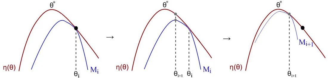 Image taken from RL — Trust Region Policy Optimization (TRPO) Explained
If M is a lower bound that never crosses η, then maximizing M must improve η.
Proof sketch:
- Since $M(\theta_{\text{old}}) = \eta(\theta_{\text{old}})$ and $M(\theta) \leq \eta(\theta)$ everywhere
- If we find $\theta_{\text{new}}$ such that $M(\theta_{\text{new}}) > M(\theta_{\text{old}})$
- Then $\eta(\theta_{\text{new}}) \geq M(\theta_{\text{new}}) > M(\theta_{\text{old}}) = \eta(\theta_{\text{old}})$
- Therefore $\eta(\theta_{\text{new}}) > \eta(\theta_{\text{old}})$ ✓
In simpler terms, we have a function $\eta(\theta)$ parameterized by $\theta$ (the weights of our neural network). It is not computationally tractable to optimize this function directly. Hence we create a close approximation function $M(\theta)$ using the lower bound function form described above. This approximation comes from the general theory of Minorize-Maximization algorithms (see Hunter & Lange, 2004).
This approximation $M(\theta)$ is computationally feasible and easier to optimize. What we have proved here is that as we improve $M(\theta)$, that improvement guarantees we also improve $\eta(\theta)$.
| By optimizing a lower bound function approximating η locally, MM guarantees policy improvement every iteration and leads us to the optimal policy eventually. |
Trust Regions
There are two major optimization paradigms:
- Line Search (like gradient descent): Choose direction first, then step size
- Trust Region: Choose maximum step size first (the size of the trust region), then find optimal point within that region
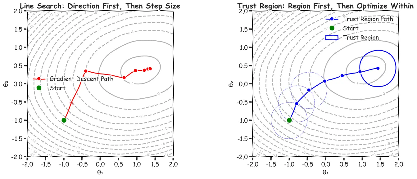
In trust region methods, we:
- Define a trust region of radius δ around current policy θ_old
- Find the optimal policy within this constrained region
- Adapt the radius based on how well our approximation worked
The optimization problem becomes: $\max_{\theta} \; M(\theta)$ $\text{subject to} \; |\theta - \theta_{old}| \leq \delta$
Adaptive Trust Region Sizing
The trust region radius δ can be dynamically adjusted:
- If approximation is good: Expand δ for next iteration
- If approximation is poor: Shrink δ for next iteration
- If policy diverges too much: Shrink δ to prevent importance sampling breakdown
Why Trust Regions Work for RL
In reinforcement learning, trust regions serve a dual purpose:
- Mathematical: Keep our quadratic approximation M valid
- Statistical: Prevent importance sampling ratios from exploding
When policies change too much, both our lower bound approximation AND our importance sampling become unreliable. Trust regions keep us in the safe zone for both.
Mathematical Notation Reference
| Symbol | Meaning |
|---|---|
| $\pi_\theta(a|s)$ | Policy probability of action a given state s |
| $\pi_{\theta_{old}}(a|s)$ | Old policy probability |
| $\tau$ | Trajectory $(s_1, a_1, s_2, a_2, \ldots)$ |
| $\pi_\theta(\tau)$ | Probability of trajectory under policy $\pi_\theta$ |
| $\frac{\pi_\theta(a_t|s_t)}{\pi_{\theta_{old}}(a_t|s_t)}$ | Importance sampling ratio for single timestep |
| $\prod_{t=1}^{T} \frac{\pi_\theta(a_t|s_t)}{\pi_{\theta_{old}}(a_t|s_t)}$ | Importance sampling ratio for full trajectory |
| $R(\tau)$ | Total reward of trajectory |
| $A(s_t, a_t)$ | Advantage function |
| $\eta(\theta)$ | Expected reward under policy $\pi_\theta$ |
| $M(\theta)$ | Lower bound function in MM algorithm |
| $\theta_{old}$ | Current policy parameters |
| $\delta$ | Trust region radius |
| $F$ | Positive definite matrix (approximating curvature) |
| $g$ | Policy gradient vector |
Trust Region Policy Optimization (TRPO)
Now we can finally understand how TRPO elegantly combines all the concepts we’ve explored:
- Importance Sampling - to reuse old data efficiently
- MM Algorithm - to guarantee policy improvement
- Trust Regions - to constrain policy changes and keep approximations valid
TRPO is a culmination of these ideas into a practical, theoretically-grounded algorithm.
Recall that our original objective was:
\[J(\pi) = \mathbb{E}_{\tau \sim \pi}[R(\tau)]\]This is the expected return (total reward) when following policy π. Instead of maximizing absolute performance $J(\pi’)$, TRPO maximizes the policy improvement:
\[\max_{\pi'} J(\pi') - J(\pi)\]This is mathematically equivalent to maximizing $J(\pi’)$ (since $J(\pi)$ is constant), but conceptually important - we’re explicitly measuring progress from our current policy.
Why focus on improvement? Because we can construct better approximations for the improvement $J(\pi’) - J(\pi)$ than for the absolute performance $J(\pi’)$. The MM algorithm works by finding lower bounds for this improvement.
To apply the MM algorithm, TRPO constructs a lower bound function ℒ that uses importance sampling:
\[\mathcal{L}_\pi(\pi') = \frac{1}{1-\gamma} \mathbb{E}_{s\sim d^\pi} \left[ \frac{\pi'(a|s)}{\pi(a|s)} A^\pi(s,a) \right] = \mathbb{E}_{\tau \sim \pi} \left[ \sum_{t=0}^{\infty} \gamma^t \frac{\pi'(a_t|s_t)}{\pi(a_t|s_t)} A^\pi(s_t, a_t) \right]\]ℒ looks complex, but let’s break this down piece by piece to understand what’s really happening here.
The discounted state visitation distribution $d^\pi(s)$ tells us how often we expect to visit each state when following policy π:
\[d^\pi(s) = (1-\gamma) \sum_{t=0}^{\infty} \gamma^t P(s_t = s|\pi)\]Think of this as a “popularity contest” for states. If γ = 1, this becomes just the regular state visit frequency under policy π. But when γ < 1, we care more about states we visit early in episodes than those we reach later. It’s like asking: “If I run my policy many times, which states will I spend most of my time in, giving more weight to earlier visits?”
The advantage function $A^\pi(s,a)$ we’ve already met - it tells us how much better taking action $a$ in state $s$ is compared to what the policy would do on average in that state.
But here’s where the magic happens. The function ℒ is essentially asking a clever question using importance sampling: “If I reweight all the actions my current policy π took according to how likely my new policy π’ would be to take them, what would my expected advantage be?”
This is brilliant because it lets us estimate how well policy π’ would perform without actually running it in the environment. We just take all our old experience from policy π and reweight it according to the probability ratio $\frac{\pi’(a|s)}{\pi(a|s)}$. When the new policy is more likely to take an action than the old one, we give that experience more weight. When it’s less likely, we give it less weight.
This importance sampling approach is what allows TRPO to reuse old data efficiently - a huge computational win over vanilla policy gradients that throw away all previous experience after each update.
The theoretical foundation comes from this crucial bound (proven in Appendix 2 of the TRPO paper):
\[J(\pi') - J(\pi) \geq \mathcal{L}_\pi(\pi') - C\sqrt{\mathbb{E}_{s\sim d^\pi}[D_{KL}(\pi' \| \pi)[s]]}\]This tells us:
- Left side: True policy improvement
- Right side: Our lower bound estimate minus a penalty term
The penalty term grows with KL divergence, so the bound becomes loose when policies differ too much.
| Consider reading this blog to get a better idea about KLD |
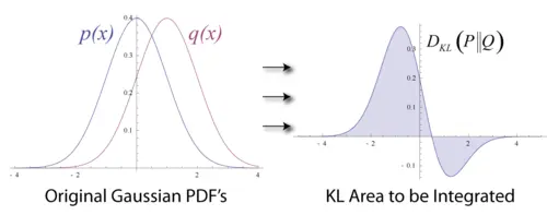 Image taken from Wikipedia
The KL divergence measures how different two probability distributions are:
\[D_{KL}(P \| Q) = \sum_x P(x) \log \frac{P(x)}{Q(x)}\]For continuous distributions, this becomes:
\[D_{KL}(P \| Q) = \int P(x) \log \frac{P(x)}{Q(x)} dx\]Think of KL divergence as asking: “If I have samples from distribution P, how surprised would I be if I thought they came from distribution Q instead?” When the distributions are identical, KL divergence is zero. As they become more different, the divergence grows.
TRPO can be formulated in two mathematically equivalent ways:
KL-Penalized (Unconstrained): \(\max_{\pi'} \mathcal{L}_\pi(\pi') - C\sqrt{\mathbb{E}_{s\sim d^\pi}[D_{KL}(\pi' \| \pi)[s]]}\)
KL-Constrained: \(\max_{\pi'} \mathcal{L}_\pi(\pi')\) \(\text{subject to } \mathbb{E}_{s\sim d^\pi}[D_{KL}(\pi'||\pi)[s]] \leq \delta\)
These formulations arise directly from the theoretical bound we mentioned earlier:
\[J(\pi') - J(\pi) \geq \mathcal{L}_\pi(\pi') - C\sqrt{\mathbb{E}_{s\sim d^\pi}[D_{KL}(\pi'||\pi)[s]]}\]The unconstrained version simply maximizes this lower bound directly. The constrained version takes a different approach: instead of penalizing large KL divergences, it prevents them entirely by adding a hard constraint.
These are mathematically equivalent due to Lagrangian duality - a beautiful result from optimization theory. For every penalty coefficient C in the unconstrained problem, there exists a constraint threshold δ in the constrained problem that gives the same optimal solution. You can think of it like this: instead of saying “I’ll pay a penalty for going over the speed limit,” you’re saying “I absolutely won’t go over the speed limit.” Both approaches can lead to the same driving behavior, just with different enforcement mechanisms.
The lower bound is what we try to maximize to find the optimum $\theta$
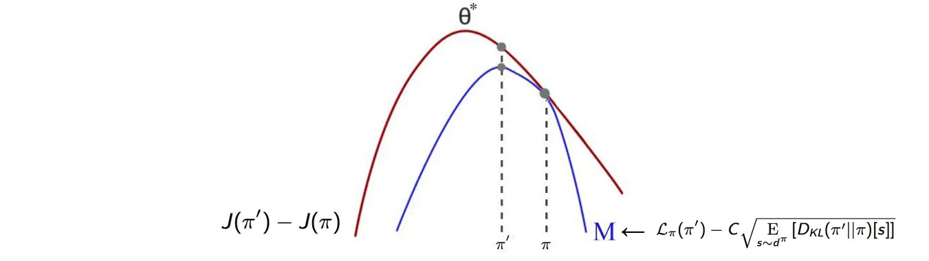 Image taken from here
However, in practice, the constrained formulation wins by a landslide. Here’s why: the penalty coefficient C becomes a nightmare to tune when the discount factor γ gets close to 1. As γ approaches 1, the coefficient explodes, making the algorithm incredibly sensitive to small changes in γ. Imagine trying to tune a parameter that changes by orders of magnitude when you adjust γ from 0.99 to 0.995 - it’s practically impossible.
\[C \propto 1/(1-\gamma)^2\]The constrained version, on the other hand, gives you direct, interpretable control. The parameter δ simply says “don’t let the policy change too much,” which is much easier to understand and tune across different environments. It’s the difference between having a thermostat that directly controls temperature versus one that requires you to calculate complex equations involving heat transfer coefficients.
| This practical insight would later inspire PPO’s breakthrough innovation. PPO took the unconstrained formulation and made it work brilliantly by replacing the complex second-order penalty with a simple first-order clipping mechanism. Instead of computing expensive Fisher Information Matrices, PPO just clips the importance sampling ratios directly - achieving similar performance with a fraction of the computational cost. |
The beauty of TRPO lies in its theoretical guarantee. Since we have the fundamental bound:
\[J(\pi') - J(\pi) \geq \mathcal{L}_\pi(\pi') - C\sqrt{\mathbb{E}_{s\sim d^\pi}[D_{KL}(\pi'(·|s) \| \pi(·|s))]}\]TRPO’s algorithm ensures three key things happen:
- Optimize $\mathcal{L}_\pi(\pi’)$ using importance sampling
- Constrain the KL divergence to stay small
- Rely on the fact that $\mathcal{L}_\pi(\pi) = 0$ when $\pi’ = \pi$
This last point is crucial and deserves explanation.
Why is ℒ_π(π) = 0? At the current policy, the importance sampling ratio becomes $\frac{\pi(a|s)}{\pi(a|s)} = 1$ for all actions. So we get:
\[\mathcal{L}_\pi(\pi) = \mathbb{E}_{s\sim d^\pi} \left[ \mathbb{E}_{a \sim \pi} \left[ 1 \cdot A^\pi(s,a) \right] \right] = \mathbb{E}_{s\sim d^\pi} \left[ \mathbb{E}_{a \sim \pi} \left[ A^\pi(s,a) \right] \right]\]But by definition, the advantage function has zero expectation under the policy - $\mathbb{E}_{a \sim \pi}[A^\pi(s,a)] = 0$ because it measures how much better each action is compared to the average. This means if we can make ℒ_π(π’) > 0 while keeping KL divergence small, we’re guaranteed that J(π’) > J(π). TRPO never moves backwards.
| You can read more about the proof here |
$\mathcal{L}_\pi(\pi’) \geq 0$ implies $J(\pi’) \geq J(\pi)$ (Our new policy will always be better or equal to our current policy)
TRPO’s guarantee: Every policy update improves performance or leaves it unchanged. We never move backwards.
Think of TRPO this way:
- Sample trajectories with current policy $\pi$
- Estimate how well any nearby policy $\pi’$ would do on these same trajectories (importance sampling)
- Find the best nearby policy within our trust region (constrained optimization)
- Verify the policy is actually better before committing (safety check)
The trust region ensures our importance sampling estimates remain accurate, while the MM algorithm structure guarantees we always improve. The constrained optimization problem: \(\max_{\pi'} \mathcal{L}_\pi(\pi')\) \(\text{subject to } \mathbb{E}_{s\sim d^\pi}[D_{KL}(\pi'||\pi)[s]] \leq \delta\)
looks intimidating, but we can solve it elegantly using a Taylor expansion around our current policy parameters θ_k. This is where the mathematical beauty of TRPO really shines through.
 Definition from Wikipedia
Let’s expand both the objective function and the constraint to second order around $\theta_k$. For the objective function $\mathcal{L}$:
Definition from Wikipedia
Let’s expand both the objective function and the constraint to second order around $\theta_k$. For the objective function $\mathcal{L}$:
Where:
- g = ∇θ Lθₖ(θ) |_θₖ (the gradient of the objective at θₖ)
- HL = ∇²θ Lθₖ(θ) |θₖ (the Hessian of the objective at θₖ)
| We can skip the terms beyond second order because they become negligibly small when $\theta$ is close to $\theta_k$. This is the fundamental assumption of trust region methods - we’re making small enough steps that higher-order terms don’t significantly affect our approximation quality. |
For the KL constraint: \(\overline{D}_{KL}(\theta|\theta_k) \approx \overline{D}_{KL}(\theta_k|\theta_k) + \nabla_\theta \overline{D}_{KL}(\theta|\theta_k)|_{\theta_k}^T (\theta - \theta_k) + \frac{1}{2}(\theta - \theta_k)^T H_{KL} (\theta - \theta_k)\)
Now comes the key insight that simplifies everything. At the current policy θ_k, several terms vanish:
- $\mathcal{L}_{\theta_k}(\theta_k) = 0$ (we showed this earlier - the advantage has zero expectation)
- $\overline{D}_{KL}(\theta_k|\theta_k) = 0$ (KL divergence of a distribution with itself is always zero)
-
∇*θ D̄_KL(θ θₖ) *θₖ = 0 (the gradient of KL divergence at the reference point is zero)
This leaves us with a beautifully clean quadratic optimization problem:
\(\max_\theta g^T (\theta - \theta_k)\) \(\text{subject to } \frac{1}{2}(\theta - \theta_k)^T H_{KL} (\theta - \theta_k) \leq \delta\)
where g is the policy gradient: \(g = \nabla_\theta \mathcal{L}_{\theta_k}(\theta) |_{\theta_k}\)
and $H_{KL}$ is the Hessian of the KL divergence, which has a special name: the Fisher Information Matrix (FIM):
\[H_{KL} = \nabla^2_\theta \overline{D}_{KL}(\theta|\theta_k) |_{\theta_k} = F = \mathbb{E}_{s,a \sim \pi_k} \left[ \nabla_\theta \log \pi_\theta(a|s) \nabla_\theta \log \pi_\theta(a|s)^T \right]\]This constrained quadratic optimization problem has a closed-form solution that can be derived using Lagrange multipliers. Setting up the Lagrangian:
\[\mathcal{L}(\theta, \lambda) = g^T (\theta - \theta_k) - \lambda \left( \frac{1}{2}(\theta - \theta_k)^T F (\theta - \theta_k) - \delta \right)\]Taking the gradient with respect to θ and setting it to zero: \(\nabla_\theta \mathcal{L} = g - \lambda F (\theta - \theta_k) = 0\)
Solving for the optimal step: \(\theta - \theta_k = \frac{1}{\lambda} F^{-1} g\)
To find λ, we substitute back into the constraint: \(\frac{1}{2} \left( \frac{1}{\lambda} F^{-1} g \right)^T F \left( \frac{1}{\lambda} F^{-1} g \right) = \delta\)
\[\frac{1}{2\lambda^2} g^T F^{-1} g = \delta\] \[\lambda = \sqrt{\frac{g^T F^{-1} g}{2\delta}}\]Putting it all together, we get the Natural Policy Gradient update:
\[\theta_{k+1} = \theta_k + \sqrt{\frac{2\delta}{g^T F^{-1} g}} F^{-1} g\]Why “Natural”? This is where things get philosophically beautiful. Regular gradient descent uses the Euclidean distance in parameter space - it treats all parameter changes as equal. But this is fundamentally wrong for probability distributions!
Consider two neural networks that represent the same policy but with different parameterizations. Vanilla gradient descent would give them different updates, even though they’re the same policy. The Natural Policy Gradient fixes this by using the Fisher Information Matrix to measure distance in the space of probability distributions rather than parameter space.
The Fisher Information Matrix captures the “curvature” of the log-likelihood surface. Areas where small parameter changes cause big changes in the policy get more weight in the distance metric. This makes the algorithm reparameterization invariant - the actual policy updates remain the same regardless of how you parameterize your neural network.
Think of it like this: if you’re navigating on a curved surface, you shouldn’t use straight-line distances to plan your path. The Fisher Information Matrix gives you the “natural” metric for that curved space, ensuring you take the most efficient steps toward better policies.
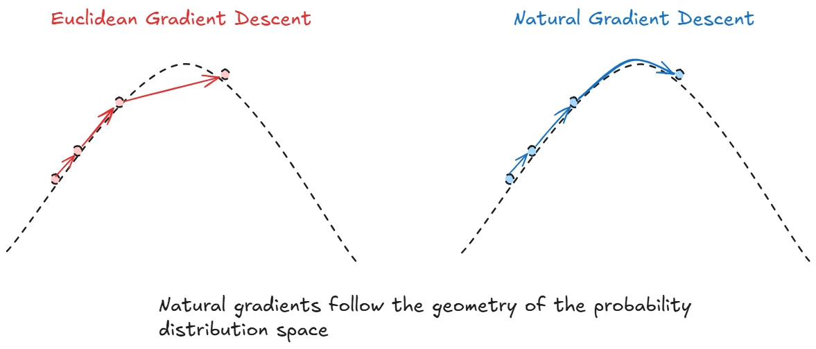
The Backtracking Line Search
Our elegant mathematical derivation gives us the Natural Policy Gradient update:
\[\theta_{k+1} = \theta_k + \sqrt{\frac{2\delta}{g^T F^{-1} g}} F^{-1} g\]But here’s the rub: this assumes our quadratic approximation is perfect. In reality, neural networks are highly nonlinear, and our Taylor expansion is only valid in a small neighborhood around $\theta_k$. The computed step might violate our KL constraint or even decrease performance when the approximation breaks down.
TRPO’s solution is beautifully practical: backtracking line search. Instead of blindly taking the full computed step, TRPO modifies the update to:
\[\theta_{k+1} = \theta_k + \alpha^j \sqrt{\frac{2\delta}{g^T F^{-1} g}} F^{-1} g\]where $\alpha \in (0, 1)$ is the backtracking coefficient (typically 0.5), and $j$ is the smallest nonnegative integer such that the new policy satisfies both:
- The KL constraint: 𝔼{s∼d^π}[D_KL(π{θ{k+1}}(·|s) ‖ π{θₖ}(·|s))] ≤ δ
- Positive improvement: ℒ{θₖ}(θ{k+1}) ≥ 0
This conservative verification ensures TRPO never violates its theoretical guarantees, even when the quadratic approximation becomes inaccurate. It’s the algorithm’s safety net - systematically reducing the step size until both conditions are met.
However, there’s a computational nightmare lurking here. The Natural Policy Gradient requires computing $F^{-1}g$, which means inverting the Fisher Information Matrix:
\[F = \mathbb{E}_{s,a \sim \pi_k} \left[ \nabla_\theta \log \pi_\theta(a|s) \nabla_\theta \log \pi_\theta(a|s)^T \right]\]For modern deep networks with millions of parameters, F is a massive n×n matrix. Computing its inverse is O(n³) - completely impractical. Even storing the full matrix requires O(n²) memory, which quickly becomes impossible for large networks.
This computational bottleneck is what led to the development of Truncated Natural Policy Gradient, and ultimately to TRPO’s clever use of conjugate gradient methods to approximate the matrix inversion without ever computing F⁻¹ explicitly.
Truncated Natural Policy Gradient
The solution to our computational nightmare is elegantly simple: instead of computing F⁻¹g directly, we use the Conjugate Gradient method to solve the linear system:
\[F x = g\]This iterative approach finds x ≈ F⁻¹g without ever computing the matrix inverse, requiring only matrix-vector products Fv. It’s like finding the solution to a puzzle without having to understand every piece - we just need to know how the pieces interact.
Conjugate Gradient works by generating search directions that are “conjugate” - meaning they’re orthogonal after being transformed by matrix F. This ensures that each new search direction doesn’t undo progress from previous iterations. For quadratic problems like ours, CG guarantees finding the exact solution in at most n steps (where n is the number of parameters), but typically converges much faster in practice.
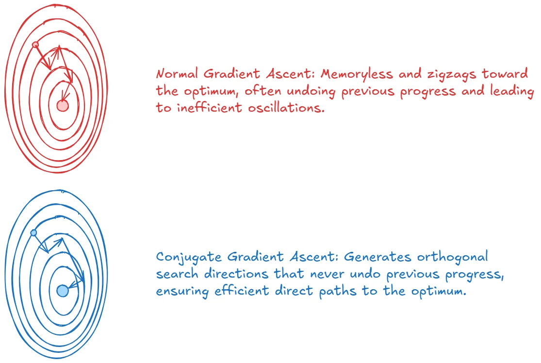
The key insight is that we never need to compute or store the full Fisher Information Matrix. Instead, we only need the matrix-vector product $Fx$ for any vector $x$. This can be computed efficiently using automatic differentiation:
\[Fx = \nabla_\theta \left( \left( \nabla_\theta \overline{D}_{KL}(\theta||\theta_k) \right)^T x \right)\]This Hessian-vector product gives us exactly what conjugate gradient needs without ever materializing the massive $F$ matrix.
The Complete TRPO Algorithm
TRPO weaves together all these concepts into a surprisingly elegant algorithm that carefully balances theoretical guarantees with practical implementation:
Step 1: Data Collection
- Collect trajectories using the current policy $\pi_k$
- Estimate the advantage function $A^{\pi_k}$ using any method (GAE, Monte Carlo returns, or temporal difference learning)
Step 2: Gradient Computation
- Compute the policy gradient \(g = \nabla_\theta \mathcal{L}_{\theta_k}(\theta) \|_{\theta_k}\)
- Set up the Fisher Information Matrix function for conjugate gradient operations
Step 3: Search Direction
- Solve $Fx = g$ using Conjugate Gradient to get the search direction $x$
- This gives us the natural gradient direction without explicitly inverting $F$
Step 4: Step Size Calculation
- Compute the initial step size to satisfy the trust region constraint
- Calculate $\alpha = \sqrt{\frac{2\delta}{g^T F^{-1} g}}$
Step 5: Conservative Verification (Line Search with Exponential Backoff)
- Propose an update: $\theta’ = \theta_k + \alpha \cdot x$
- Verify two critical conditions:
- KL divergence constraint: \(\mathbb{E}_{s\sim d^\pi}[D_{KL}(\pi'(·\|s) \| \pi(·\|s))] \leq \delta\)
- Surrogate improvement: $\mathcal{L}_{\theta_k}(\theta’) \geq 0$
- If either verification fails: reduce $\alpha$ (typically by half) and try again
- Only commit to the policy update after both conditions are satisfied
This conservative approach guarantees the theoretical properties we derived, but it also reveals TRPO’s fundamental tension between theory and practice. The algorithm is theoretically beautiful but computationally demanding, requiring multiple verification steps and potential backtracking that can make each update quite expensive.
TRPO’s Limitations
Despite its theoretical elegance, TRPO faces several practical challenges that motivated simpler alternatives:
- Computational Overhead: Computing Fisher Information Matrices and running conjugate gradient makes each update significantly more expensive than first-order methods like Adam
- Sample Inefficiency: Requires large batch sizes to accurately estimate the FIM - small batches lead to noisy estimates and unstable training
- Scalability Issues: Second-order computations become impractical for very large neural networks where first-order methods excel
TRPO’s story represents a classic tension in machine learning: the trade-off between theoretical rigor and practical utility. While TRPO provided crucial theoretical insights about policy optimization - principled policy updates, trust region concepts, and guaranteed improvement - its computational complexity limited its real-world impact.
This limitation sparked a natural question: could we achieve similar performance guarantees with a much simpler algorithm? The answer would come in the form of Proximal Policy Optimization (PPO), which took TRPO’s core insights and packaged them into an algorithm so simple and effective that it would become the workhorse of modern policy optimization.
As we noted earlier from the PPO paper: “Q-learning (with function approximation) fails on many simple problems and is poorly understood, vanilla policy gradient methods have poor data efficiency and robustness; and trust region policy optimization (TRPO) is relatively complicated, and is not compatible with architectures that include noise (such as dropout) or parameter sharing.”
PPO’s breakthrough was recognizing that you don’t need complex second-order methods to implement trust regions effectively. Instead of computing Fisher Information Matrices and running conjugate gradient, PPO simply clips the importance sampling ratios directly. This first-order approach achieves similar practical performance while being orders of magnitude simpler to implement and debug.
Note: TRPO in a crux is simple, it is a constrained optimization problem. To solve which we need second order derivatives. Which is computationally expensive and no current ML framework solves it without significant overhead. But do know, it is a tough topic to truly understand. One needs to be well-versed with many prerequisite mathematical knowledge. Do not be dishearted if it takes you time to understand it thorougly. Read slowly, daily, iteratively.
Proximal Policy Optimization (PPO)
PPO emerged from a simple observation: what if we could achieve TRPO’s stability guarantees without all the computational complexity? The genius of PPO lies in replacing TRPO’s hard KL constraint with a clever objective function that naturally prevents large policy updates.
Let’s first understand the core innovation. Remember TRPO’s constrained optimization problem:
\[\max_{\theta} \mathcal{L}_{\theta_{old}}(\theta) \quad \text{subject to } \mathbb{E}_{s \sim d^{\pi_{old}}}[D_{KL}(\pi_{old}(\cdot|s) || \pi_\theta(\cdot|s))] \leq \delta\]PPO asks: instead of explicitly constraining the KL divergence, what if we modify the objective function itself to penalize large policy changes? This transforms a constrained optimization problem into an unconstrained one that standard optimizers like Adam can handle.
The Clipped Surrogate Objective
PPO introduces a brilliantly simple idea. Define the probability ratio:
\[r_t(\theta) = \frac{\pi_\theta(a_t|s_t)}{\pi_{\theta_{old}}(a_t|s_t)}\]This ratio tells us how much more (or less) likely the new policy is to take the same action compared to the old policy. When $r_t(\theta) = 1$, the policies agree perfectly. When $r_t(\theta) = 2$, the new policy is twice as likely to take that action.
The vanilla policy gradient objective using importance sampling would be:
\[L^{IS}(\theta) = \mathbb{E}_t[r_t(\theta) \cdot A_t]\]But this can lead to destructively large policy updates when $r_t(\theta)$ becomes very large or very small. PPO’s innovation is to clip this ratio:
\[L^{CLIP}(\theta) = \mathbb{E}_t[\min(r_t(\theta) \cdot A_t, \text{clip}(r_t(\theta), 1-\epsilon, 1+\epsilon) \cdot A_t)]\]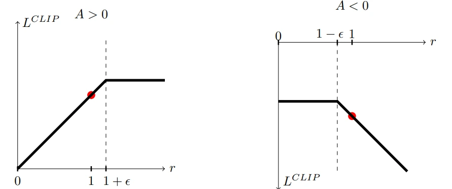 Image taken from paper
Let’s unpack this equation with concrete examples to build intuition.
Case 1: Positive Advantage (A_t > 0)
When an action led to better-than-expected rewards, we want to increase its probability. Let’s say $A_t = 2$ and $\epsilon = 0.2$.
-
If $r_t(\theta) = 0.5$ (new policy half as likely):
- Unclipped objective: $0.5 \times 2 = 1$
- Clipped objective: $\min(1, 0.8 \times 2) = 1$
- No clipping occurs since we’re making the policy worse for a good action
-
If $r_t(\theta) = 1.5$ (new policy 50% more likely):
- Unclipped objective: $1.5 \times 2 = 3$
- Clipped objective: $\min(3, 1.2 \times 2) = 2.4$
- Clipping kicks in! We cap the improvement to prevent overconfidence
The key insight: for positive advantages, clipping prevents us from changing the policy too aggressively in the “good” direction. Once $r_t(\theta) > 1 + \epsilon$, there’s no benefit to increasing it further.
Case 2: Negative Advantage (A_t < 0)
When an action led to worse-than-expected rewards, we want to decrease its probability. Let’s say $A_t = -2$ and $\epsilon = 0.2$.
-
If $r_t(\theta) = 0.5$ (new policy half as likely):
- Unclipped objective: $0.5 \times (-2) = -1$
- Clipped objective: $\min(-1, 0.8 \times (-2)) = -1.6$
- Clipping makes the objective more negative, encouraging further reduction
-
If $r_t(\theta) = 1.5$ (new policy 50% more likely):
- Unclipped objective: $1.5 \times (-2) = -3$
- Clipped objective: $\min(-3, 1.2 \times (-2)) = -3$
- No clipping since we’re increasing probability of a bad action
For negative advantages, clipping prevents us from reducing the probability too aggressively. Once $r_t(\theta) < 1 - \epsilon$, there’s no benefit to decreasing it further.
The Mathematical Beauty of PPO’s Objective
The clipped objective creates a “trust region” implicitly. When the policy changes too much (beyond $1 \pm \epsilon$), the gradient of the clipped objective becomes zero with respect to $\theta$. This elegant mechanism automatically prevents destructive updates without requiring second-order optimization.
To see this mathematically, consider the gradient when $A_t > 0$ and $r_t(\theta) > 1 + \epsilon$:
\[\frac{\partial L^{CLIP}}{\partial \theta} = \frac{\partial}{\partial \theta}[\text{clip}(r_t(\theta), 1-\epsilon, 1+\epsilon) \cdot A_t] = 0\]The gradient vanishes because the clipped value $(1+\epsilon)$ doesn’t depend on $\theta$. This creates a “flat” region in the loss landscape that prevents further movement in that direction.
PPO with Adaptive KL Penalty
Before arriving at the clipped objective, the PPO paper explored a KL penalty approach that directly connects to TRPO:
\[L^{KLPEN}(\theta) = \mathbb{E}_t[r_t(\theta) \cdot A_t - \beta \cdot D_{KL}(\pi_{\theta_{old}}(\cdot|s_t) || \pi_\theta(\cdot|s_t))]\]This is exactly the unconstrained version of TRPO’s problem! The Lagrangian of TRPO’s constrained optimization:
\[\max_{\theta} \mathcal{L}_{\theta_{old}}(\theta) - \lambda(\mathbb{E}[D_{KL}] - \delta)\]becomes PPO’s KL penalty objective when we fix $\beta = \lambda$. The key difference: PPO adapts $\beta$ dynamically during training:
if kl_divergence > 1.5 * target_kl:
    beta *= 2  # Increase penalty
elif kl_divergence < target_kl / 1.5:
    beta /= 2  # Decrease penalty
However, this adaptive mechanism proved finicky in practice. The clipped objective achieved similar goals with fixed hyperparameters, making it the preferred approach.
Why Multiple Epochs Work: The Importance Sampling Perspective
A subtle but crucial aspect of PPO is performing multiple epochs of updates on the same data. This seems to violate our earlier concern about importance sampling breaking down when policies diverge. The clipping mechanism is precisely what makes this safe.
Consider what happens over multiple epochs:
- Epoch 1: Policy changes slightly, ratios stay near 1
- Epoch 2: For trajectories where policy already changed, clipping prevents further movement
- Epochs 3-10: Most gradients are zero due to clipping, only “unexploited” trajectories contribute
The clipping essentially creates a curriculum where different parts of the data become “active” in different epochs, naturally preventing overfitting to any particular trajectory.
PPO’s clipping prevents the fine-tuned model from diverging too far from the base model’s distribution, maintaining fluency while optimizing for human preferences. This is why responses from RLHF models feel coherent - they’re constrained to stay within a trust region of the original model’s behavior.
The journey from policy gradients through TRPO to PPO represents a beautiful example of how complex theoretical insights can be distilled into simple, practical algorithms. PPO takes TRPO’s guarantee of monotonic improvement and approximates it with a first-order method that captures the essential insights: prevent destructive updates, enable data reuse, and maintain computational simplicity.
MoE
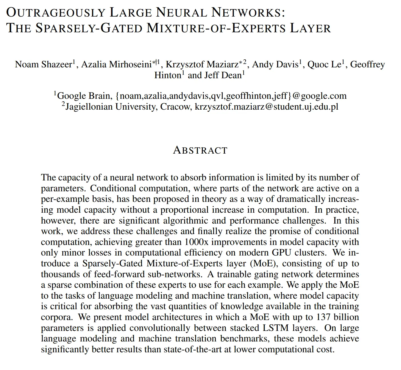
Link to paper: Outrageously Large Neural Networks: The Sparsely-Gated Mixture-of-Experts Layer
Link to implementation: [WORK IN PROGRESS]
Quick Summary
This 2017 paper by Shazeer et al. introduces a novel approach to dramatically increase neural network capacity without proportionally increasing computational costs. The core innovation is the Sparsely-Gated Mixture-of-Experts (MoE) layer, which contains thousands of feed-forward neural networks (experts), with a trainable gating network that selectively activates only a small subset of experts for each input example.
Key highlights:
- The authors achieve over 1000x improvements in model capacity while maintaining computational efficiency
- Their approach addresses several challenges of conditional computation, including GPU utilization and load balancing
- When applied to Language Modeling and machine translation tasks, their MoE models significantly outperform state-of-the-art models with lower computational cost
- Their largest model contains up to 137 billion parameters and demonstrates continued performance improvements with increased capacity
This paper represents a significant advancement in scaling neural networks efficiently, presaging some of the techniques that would later become important in very large language models.
Another explosive paper, in 2017. Talk about being a crazy year right. Well to be perfectly honest MOE was actually introduced in 1991 in the paper Adaptive Mixture of Local Experts. But Noam et al introduced the idea to LSTMs, which really blew up.
Problem
The capacity of a neural network to absorb information is limited by its number of parameters.
Solution
Conditional computation, where parts of the network are active on a per-example basis, has been proposed in theory as a way of dramatically increasing model capacity without a proportional increase in computation.
The following blogs helped me immensely while writing this section
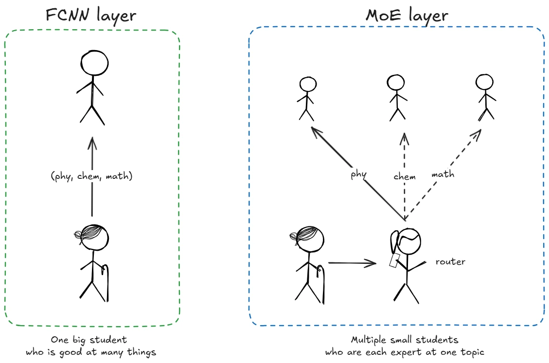
A simple intuition behind MoE can be seen as above, A single dense neural network is like a big student. Who has general knowledge about a lot of things without being particularly great at any one topic. When you ask him a question he takes his time to think and answers you, He also eats a lot because he is big.
But with a MoE layer, a smart router reads the question and directs it to the right expert. That expert gives a focused answer since they only need to worry about their specialty. As we’re only activating one small expert instead of the entire large model, we use much less computation while still having access to lots of specialized knowledge.
The above visualization is good for intuition point of view, but that is not how MoEs actually work in practice. For starter each expert is not an expert in a topic but expert in tokens, some can be punctuation experts, some can be noun experts etc.(More on this later)
This work introduced MoEs to LSTMs, so let us proceed forward in understanding that. Consider reading the following blog Understanding LSTM Networks by Christopher Olah & Recurrent Neural Networks (RNNs), Clearly Explained!!! by Josh Starmer if you need a refresher on the topic.

In an MoE model, the Fully connected neural network(FCNN) (Or the hiddens state in case of RNNs & LSTMs) is replaces with an MoE layer. The MoE layer consists of a gating function which outputs a probability distribution of likely experts. The experts themselves are smaller FCNN. The output of the experts is multiplied with their probability after which it is finally summed over.
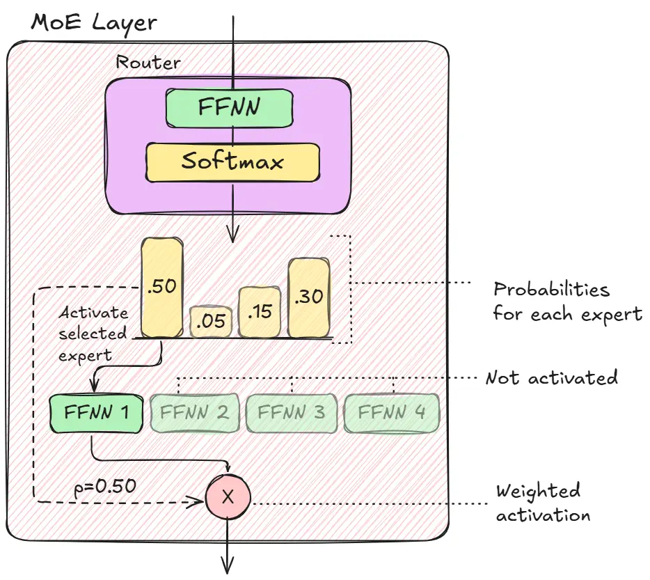
The idea seems simple enough, but there are multiple complexities like:
- How do you create a fair gating function?
- How many experts do you choose?
- How many tokens do you send to each expert?
Let’s us go through each question one by one.
Note: We will see many changes that were made on this idea as we progress, but this was the foundational paper on MoEs for large models. So it is crucial that you understand it well.
Sparse vs Dense Networks
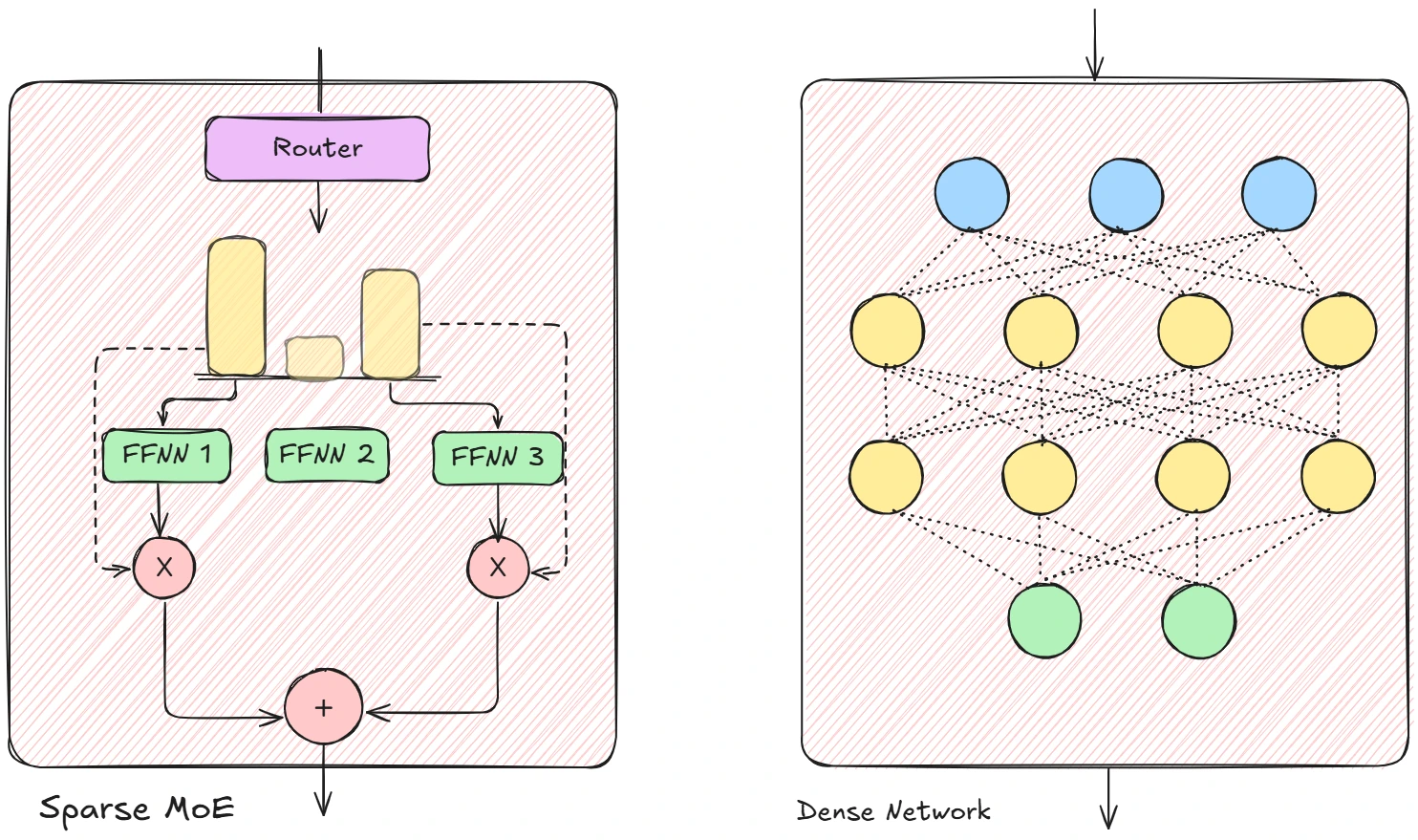
Dense Networks: Every parameter is used for every input
- High computational cost that scales linearly with parameters
- Limited by memory and compute constraints
- Parameters must be “generalists” handling all types of inputs
Sparse Networks (MoE): Only a subset of parameters are used per input
- Computational cost scales with active experts, not total experts
- Can have 1000x more parameters with similar compute budget
- Parameters can be highly specialized for specific patterns
conditional computation allows us to scale model capacity without proportional compute scaling. It’s like having a library with thousands of specialized books, but only reading the few relevant ones for each question.
The Gating Network
First let us understand how the output is calculated in a sparse MoE.
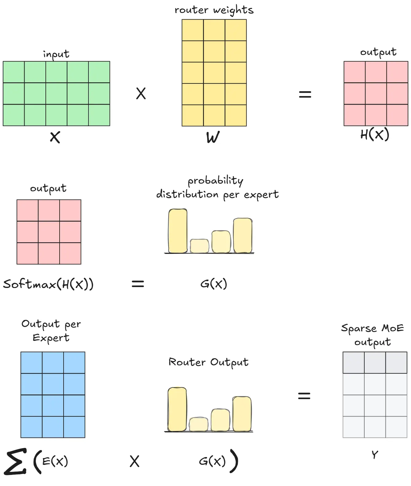
We begin with an input matrix X, multiple that by the router weights W. We take the softmax of this output to get the probability distribution $G(x)$. This is the likelihood of which experts are best for the given input.
Depending on how many experts we choose, we take the output of those experts and multiply that with the probability of that output begin chosen (This is done distriute the importance of the output based on which expert is most likely to be chosen). That gives us the output.
When we put it all together, this is how it looks.
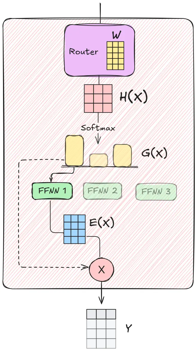
The original paper introduced two key innovations:
Softmax Gating (Dense Baseline)
# Simple dense gating - activates ALL experts with different weights
G(x) = Softmax(x · W_g)
y = Σ G(x)_i * Expert_i(x)  # All experts contribute
Noisy Top-K Gating (The Sparse Innovation)
# Step 1: Add trainable noise for load balancing
H(x)_i = (x · W_g)_i + StandardNormal() * Softplus((x · W_noise)_i)

# Step 2: Keep only top K experts, set others to -∞
KeepTopK(v, k)_i = {
    v_i    if v_i is in top k elements
    -∞     otherwise
}

# Step 3: Apply softmax (experts with -∞ get probability 0)
G(x) = Softmax(KeepTopK(H(x), k))
Why the noise? The Gaussian noise helps with load balancing. Without it, the same few experts would always dominate, creating a “rich get richer” problem where popular experts get more training and become even more popular.
Why Top-K? By keeping only the top K experts (typically K=2 or K=4), we achieve:
- Sparsity: Most experts are inactive, saving computation
- Specialization: Each expert focuses on specific patterns
- Scalability: We can add thousands of experts without proportional compute increase
Addressing Performance Challenges
The paper identified several critical challenges that needed solving for MoE to work in practice:
The Shrinking Batch Problem
Original batch: 1024 examples
With 256 experts, k=4: Each expert sees only ~16 examples
Small batches = inefficient GPU utilization
Solution:
Mix Data and Model Parallelism
- Combine batches from multiple GPUs before sending to experts
- Each expert gets larger effective batch size:
(batch_size * num_devices * k) / num_experts - Achieves factor of
dimprovement in expert batch size withddevices
Network Bandwidth Bottleneck
Modern GPUs have computational power thousands of times greater than network bandwidth. Meaning most time is spent between I/O operations.
Solution:
- Keep experts stationary on devices (don’t move the experts)
- Only send inputs/outputs across network (much smaller)
- Use larger hidden layers to improve computation-to-communication ratio
| To understand this better, consider reading Making Deep Learning Go Brrrr From First Principles |
Load Balancing Problem
Without intervention, a few experts dominate while others are rarely used. This creates a vicious cycle: popular experts get more training data, become better, and thus get selected even more often. Meanwhile, neglected experts remain undertrained and essentially become dead weight.
Think of it like a classroom where only the brightest students get called on - they get more practice and become even brighter, while others stagnate.
The Dual Challenge
The paper identifies that we need to balance two distinct but related problems:
- Importance Imbalance: Some experts get high gating weights but few examples
- Load Imbalance: Some experts get many examples but low individual weights
Both scenarios are problematic. An expert with few high-weight examples overfits to specific patterns, while an expert with many low-weight examples receives weak learning signals.
Mathematical Solution: Auxiliary Loss
The authors introduce a load balancing loss that uses the coefficient of variation (CV) to measure and penalize imbalance:
\[CV = \frac{\sigma}{\mu} = \frac{\text{standard deviation}}{\text{mean}}\]The CV is beautiful because it’s scale-invariant - it measures relative variability regardless of the absolute magnitudes. A CV of 0 means perfect balance, while higher values indicate increasing imbalance.
Step 1: Measuring Importance
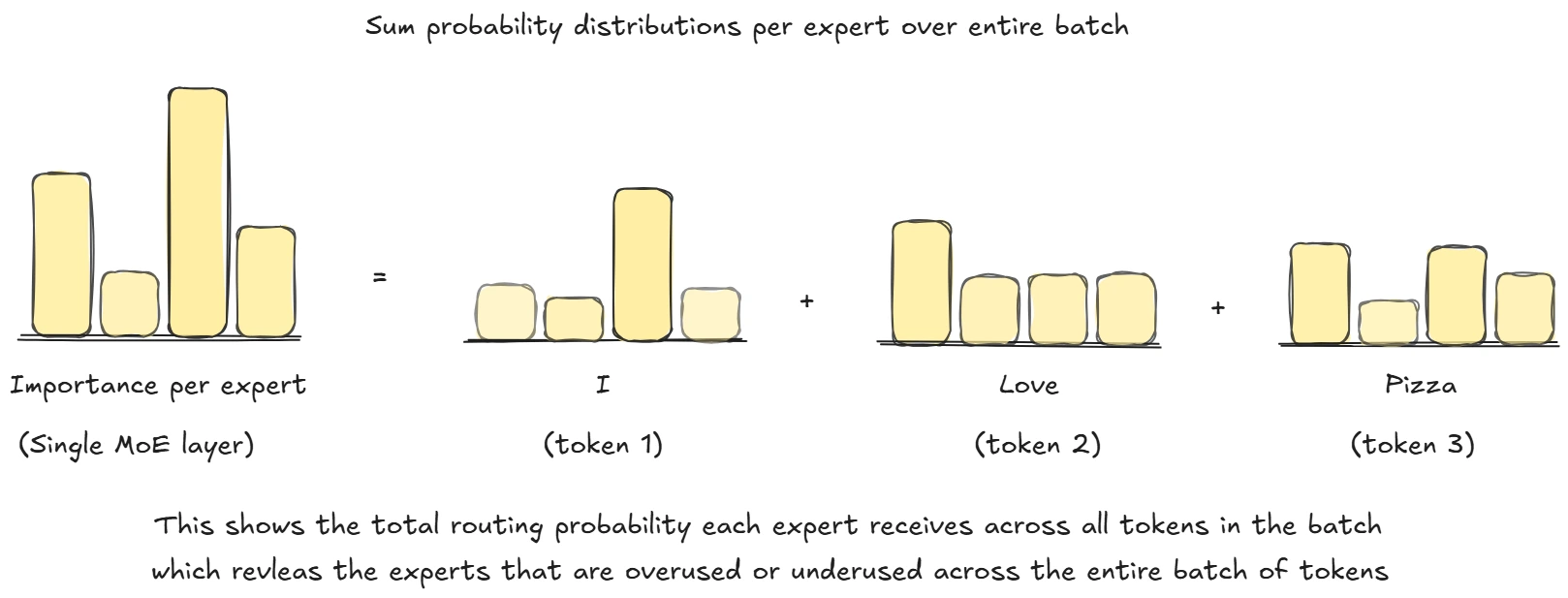
For each expert $i$, we sum its gating probabilities across the entire batch:
\[\text{Importance}(X)_i = \sum_{x \in X} G(x)_i\]This gives us the “importance scores” - how much each expert contributes regardless of which specific examples it processes.
Step 2: Computing the Importance Loss
\[\mathcal{L}_{\text{importance}} = w_{\text{importance}} \cdot CV(\text{Importance}(X))^2\]Where: \(CV(\text{Importance}(X)) = \frac{\sigma(\text{Importance}(X))}{\mu(\text{Importance}(X))}\)
Why square the CV? This creates a stronger penalty for large imbalances and makes the gradient more well-behaved during optimization.
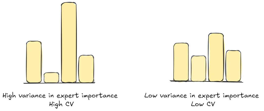
Step 3: Measuring Load
Load measures how many examples each expert actually processes:
\[\text{Load}(X)_i = \sum_{x \in X} \mathbf{1}[\text{expert } i \text{ is in top-k for } x]\]In practice, this uses a smooth differentiable approximation rather than the hard indicator function.
Step 4: Computing the Load Loss
\[\mathcal{L}_{\text{load}} = w_{\text{load}} \cdot CV(\text{Load}(X))^2\]The Complete Auxiliary Loss
\[\mathcal{L}_{\text{auxiliary}} = w_{\text{importance}} \cdot CV(\text{Importance}(X))^2 + w_{\text{load}} \cdot CV(\text{Load}(X))^2\]Final Training Objective
\[\mathcal{L}_{\text{total}} = \mathcal{L}_{\text{main}} + \mathcal{L}_{\text{auxiliary}}\]Why Both Losses Matter
Consider these scenarios:
- Expert A: Gets selected for 100 examples with average weight 0.01 each
- Expert B: Gets selected for 2 examples with average weight 0.5 each
- Expert C: Gets selected for 50 examples with average weight 0.02 each
All have similar total importance (≈ 1.0), but vastly different training dynamics:
- Expert A gets many weak signals → slow learning
- Expert B gets few strong signals → overfitting risk
- Expert C gets balanced signal → healthy learning
The dual loss ensures both the total contribution (importance) and the number of training examples (load) are balanced across experts.
Practical Impact
With proper load balancing:
- All experts receive sufficient training signal
- No expert dominates the computation
- Model capacity is fully utilized
- Training stability improves dramatically
This auxiliary loss was crucial for making MoE work at scale - without it, the models would collapse to using only a handful of experts, defeating the entire purpose of conditional computation.
Expert Capacity

This wasn’t introduced in this paper, but let’s talk about it too since it’s crucial for modern MoE implementations. Even with perfect load balancing, there’s another challenge: token overflow. In the example above, FFNN 1 receives the majority of tokens. To prevent any single expert from being overwhelmed, we set an Expert Capacity - a maximum number of tokens each expert can process per batch. When an expert reaches capacity, additional tokens that would have been routed to it are either sent to the next-best expert or bypass the MoE layer entirely (called token overflow). This capacity mechanism ensures balanced computational load across experts and prevents memory bottlenecks, though it can sometimes mean tokens don’t get processed by their optimal expert. The trade-off between perfect routing and practical constraints is a key engineering challenge in scaling MoE systems.
Training the MoE Model
Key Challenge: How do experts specialize without explicit supervision?
The specialization emerges through training dynamics:
- Initial randomness: All experts start random and perform similarly
- Noise-induced preferences: The noise in gating creates slight preferences
- Reinforcement loop: Experts that perform well for certain inputs get selected more
- Emergent specialization: Through this process, experts develop distinct capabilities
What do experts actually learn? (From the paper’s analysis)
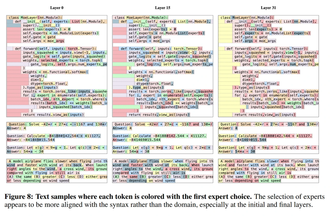 Image taken from Mistral paper
Unlike the intuitive “biology expert” or “math expert”, real MoE experts learn much more fine-grained patterns:
- Syntactic specialization: Expert 381 specializes in contexts with “researchers”, “innovation”, and “technology”
- Positional patterns: Expert 752 handles phrases where indefinite article “a” introduces important concepts
- Semantic clustering: Expert 2004 focuses on contexts involving speed and rapid change
This emergent specialization is what makes MoE powerful - experts automatically discover useful divisions of labor without being explicitly told what to specialize in.
Revolutionary Results
Language Modeling (1B Word Benchmark):
- 4096-expert MoE: 24% better perplexity than dense baseline
- Same computational cost as much smaller dense models
- Up to 137B parameters (1000x parameter increase) with minimal compute overhead
- Training time: 12 hours vs weeks for equivalent dense models
Machine Translation (WMT’14):
- En→Fr: 40.56 BLEU (vs 39.22 for GNMT)
- En→De: 26.03 BLEU (vs 24.91 for GNMT)
- Achieved new state-of-the-art with lower computational cost
- Faster training than dense models with better quality
Computational Efficiency:
- MoE models achieved 0.74-1.56 TFLOPS/GPU
- Significant fraction of theoretical maximum (4.29 TFLOPS/GPU)
- Only 37-46% of operations were in expert computations
The Breakthrough: This was the first time conditional computation delivered on its theoretical promise at scale. Previous attempts had struggled with the practical challenges that this paper solved.
From LSTMs to Modern Transformers
While this paper applied MoE to LSTMs (the dominant architecture in 2017), the core insights proved even more powerful when later applied to Transformers, about which we will learn more about in the later sections.
The path from this 2017 paper to modern LLMs shows how foundational ideas can have delayed but massive impact. Key lessons that influenced later work:
- Sparsity enables scale: The core insight that you can have orders of magnitude more parameters without proportional compute increase
- Load balancing is crucial: Without proper load balancing, MoE models fail to train effectively
- Engineering matters: Success required solving practical challenges like communication costs and batch sizing
- Specialization emerges: Given proper training dynamics, experts will naturally develop useful specializations
Today’s largest language models increasingly rely on MoE architectures, making this paper’s contributions more relevant than ever. The ability to scale to trillion-parameter models while maintaining reasonable training costs has become essential for pushing the boundaries of AI capabilities.
2018: BERT and Early Innovations
ULMFiT
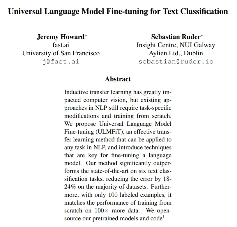
Link to paper: Universal Language Model Fine-tuning for Text Classification
Quick Summary
This 2018 paper by Jeremy Howard and Sebastian Ruder introduces ULMFiT (Universal Language Model Fine-tuning), a method for transfer learning in NLP tasks. The authors present an approach that mirrors the success of transfer learning in computer vision by using a pre-trained language model and fine-tuning it for specific text classification tasks.
Key contributions:
-
A three-stage approach to transfer learning for NLP tasks:
- General-domain language model pretraining
- Target task language model fine-tuning
- Target task classifier fine-tuning
-
Novel fine-tuning techniques to prevent catastrophic forgetting:
- Discriminative fine-tuning (using different learning rates for different layers)
- Slanted triangular learning rates (a specific learning rate schedule)
- Gradual unfreezing (progressively unfreezing layers from last to first)
-
State-of-the-art results on six text classification datasets with significant error reductions (18-24%)
-
Impressive sample efficiency - with just 100 labeled examples, the method matches the performance of training from scratch with 10-100x more data
The paper demonstrates that effective transfer learning is possible in NLP without task-specific modifications or architecture changes, using a standard 3-layer LSTM model with careful fine-tuning techniques.
It is unfortunate that such an amazing paper which was a direct influence on the way GPT-1 was trained is often not talked about enough when it comes to LLM. Let’s do justice to that and understand more about Universal Language Model Fine-tuning or ULMFiT!!!
Problem
Inductive transfer learning has greatly impacted computer vision, but existing approaches in NLP still require task-specific modifications and training from scratch.
Before ULMFiT, transfer learning in NLP had a fatal flaw: catastrophic forgetting. When you fine-tuned a pretrained model on a new task, the model would rapidly “forget” its pretrained knowledge and overfit to the small target dataset. It was like teaching a polyglot to speak a new dialect, only to watch them forget all their other languages in the process.
This made transfer learning frustrating and often counterproductive. Researchers would get excited about pretrained models, only to find that fine-tuning destroyed the very knowledge they wanted to leverage.
Solution
ULMFiT, an effective transfer learning method that can be applied to any task in NLP, and introduce techniques that are key for fine-tuning a language model.
This paper laid crucial groundwork for the LLM revolution we see today.
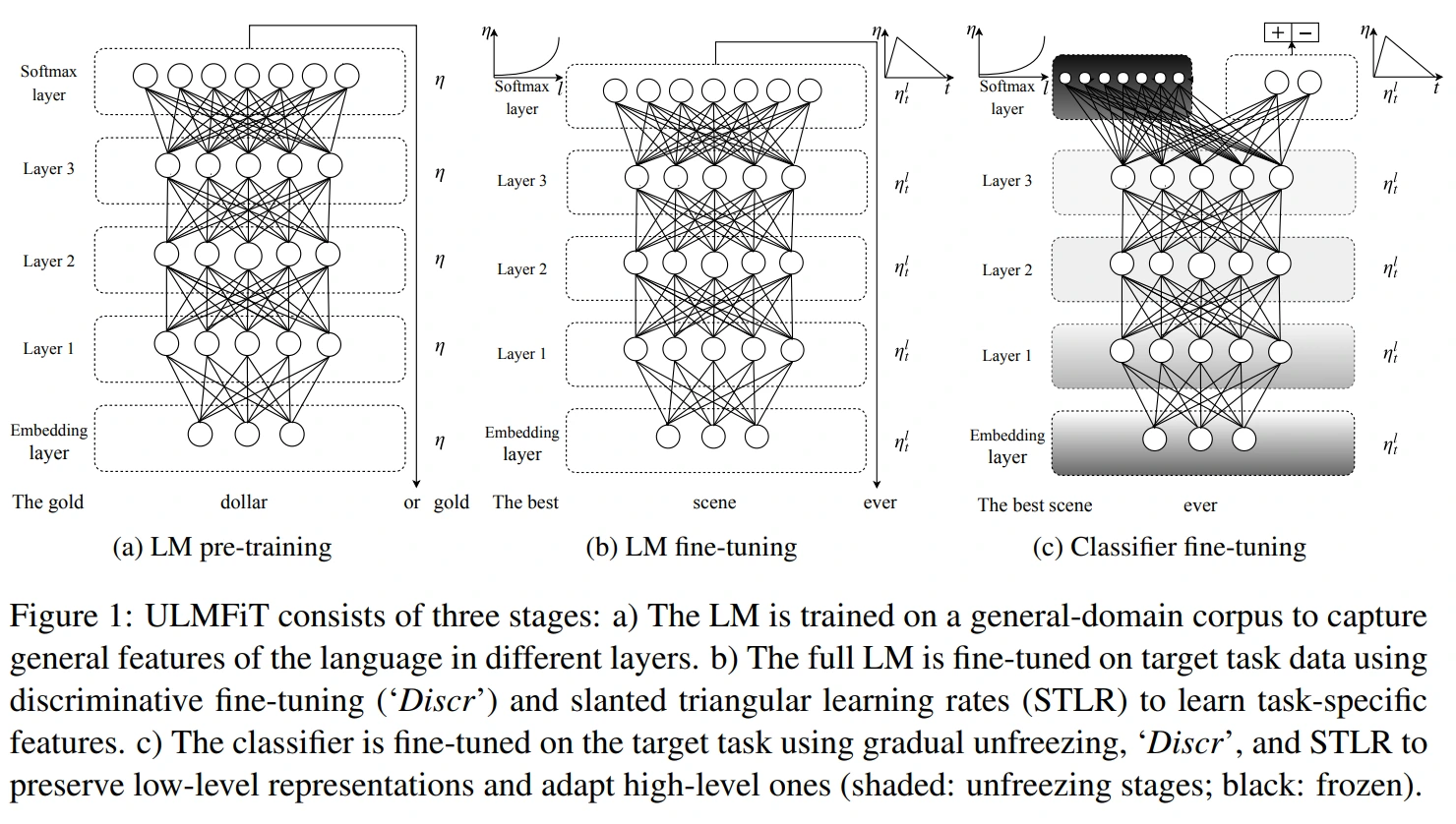
The first stage is pretty basic and nothing innovative, but the second & third stage is where the innovation lies.
So far noone had been able to fine tune a general purpose model to perform well on target task which was not present in the original modeling of the original model
Why Transfer Learning Failed in NLP
Unlike computer vision, where you could take ImageNet features and achieve great results on new tasks, NLP models seemed to resist transfer. The problem wasn’t the models themselves but how we fine-tuned them. Traditional approaches used the same learning rate for all layers and froze nothing, causing rapid degradation of learned representations. ULMFiT’s breakthrough was realizing that different layers need different treatment during fine-tuning.
Let us understand each stage one by one
1st stage: General-domain LM pretraining
This is the simplest albeit the most expensive stage. Take a large dataset that has general information on many topics and train your model on it.
“We pretrain the language model on Wikitext-103 (Merity et al., 2017b) consisting of 28,595 preprocessed Wikipedia articles and 103 million words.”
This helps the model learn general language properties, At this stage it is nothing more than a really good next token predictor.
For example if you asked it the question
“What is the capital of France?”
Instead of getting Paris as the answer you will get. “What is the capital of India ?What is the captial of China” and so on.
That is where the innovative “fine-tuning” part comes in.
2nd Stage: Target task Language Model fine-tuning
Fine-tuning let us teach the LLM to follow our task specific requirements and control it’s behaviour in our target dataset.
Discriminative fine-tuning
In any deep neural network, different layers capture different parts of the dataset (This is a very popular article visualizing different parts of a CNN model). So it is reasonable to think that it won’t be a good idea to use the same learning rate to fine-tune each layer.
That is the idea behind discriminative fine-tuning. In this we have a different learning rate for each layer.
Stochastic Gradient Descent
\[\theta_t = \theta_{t-1} - \eta \cdot \nabla_\theta J(\theta)\]Stochastic Gradient Descent with different learning rate for each layers
\[\theta_t^l = \theta_{t-1}^l - \eta^l \cdot \nabla_{\theta^l} J(\theta)\]The authors found that it’s best to first find the optimum $\eta^L$ for the last layer, then go downstream following this rule $\eta^{l-1} = \eta^l/2.6$
Slanted triangular learning rates
When fine-tuning a pretrained model, we face a fundamental tension. We want the model to quickly adapt to our target task, but we also need to preserve the valuable knowledge it learned during pretraining. Fixed learning rates can’t solve this dilemma.
To solve that the authors introduced STLR, an adaptive learning rate that changes with number of iterations.
The idea is, start with a higher learning rate to rapidly adapt the model to the target task’s patterns, then gradually decrease it to fine-tune without destroying pretrained representations.
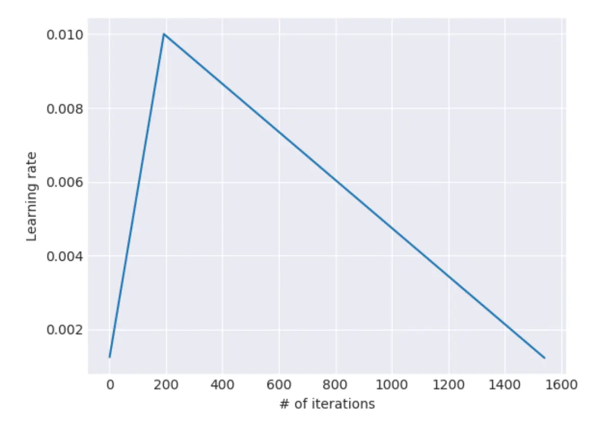
Think of it like learning to drive in a new city. Initially, you drive faster to quickly get oriented and find the general area you need. Once you’re close to your destination, you slow down to carefully navigate the final streets and parking.
This was achieved using the following formula
\[\text{cut} = \lfloor T \cdot \text{cut\_frac} \rfloor\] \[p = \begin{cases} t/\text{cut}, & \text{if } t < \text{cut} \\ 1 - \frac{t-\text{cut}}{\text{cut} \cdot (1/\text{cut\_frac} - 1)}, & \text{otherwise} \end{cases}\] \[\eta_t = \eta_{\max} \cdot \frac{1 + p \cdot (\text{ratio} - 1)}{\text{ratio}}\]Where:
- $T$ is the total number of training iterations
- $\text{cut_frac}$ is the fraction of iterations for learning rate increase (typically 0.1)
- $\text{cut}$ is the iteration where we switch from increasing to decreasing
- $p$ is the fraction of iterations in current phase
- $\text{ratio}$ specifies how much smaller the lowest LR is from maximum (typically 32)
- $\eta_{\max}$ is the maximum learning rate (typically 0.01)
- $\eta_t$ is the learning rate at iteration $t$
3rd Stage: Target task classifier fine-tuning
The final stage adds a classifier head to the fine-tuned language model and trains it for the specific task. This stage introduces several crucial techniques that prevent the model from forgetting its pretrained knowledge.
Gradual Unfreezing
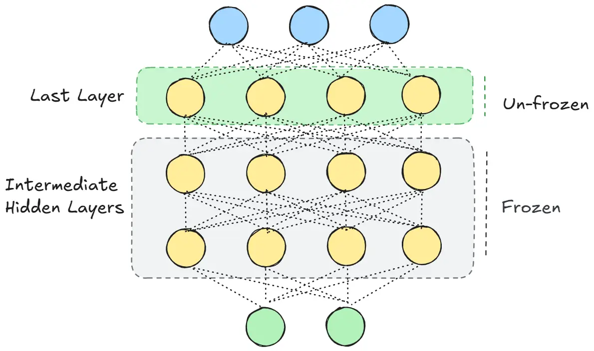
Rather than fine-tuning all layers at once, which risks catastrophic forgetting, ULMFiT gradually unfreezes layers starting from the last layer. The intuition is elegant: the last layers contain the most task-specific knowledge, while early layers capture universal language features that should change slowly.
The process works like this: First, unfreeze only the classifier head and train for one epoch. Then unfreeze the next layer down and continue training. Repeat this process until all layers are unfrozen. This gradual approach gives the model time to adapt each layer’s representations smoothly without destroying the foundation built in earlier layers.
Concat Pooling
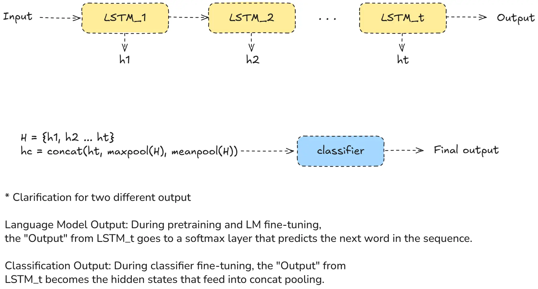
ULMFiT also introduced concat pooling for text classification. Instead of using only the final hidden state, it concatenates the last hidden state with both max-pooled and mean-pooled representations across all timesteps. This captures information from the entire document, not just the end.
BPTT for Text Classification (BPT3C)
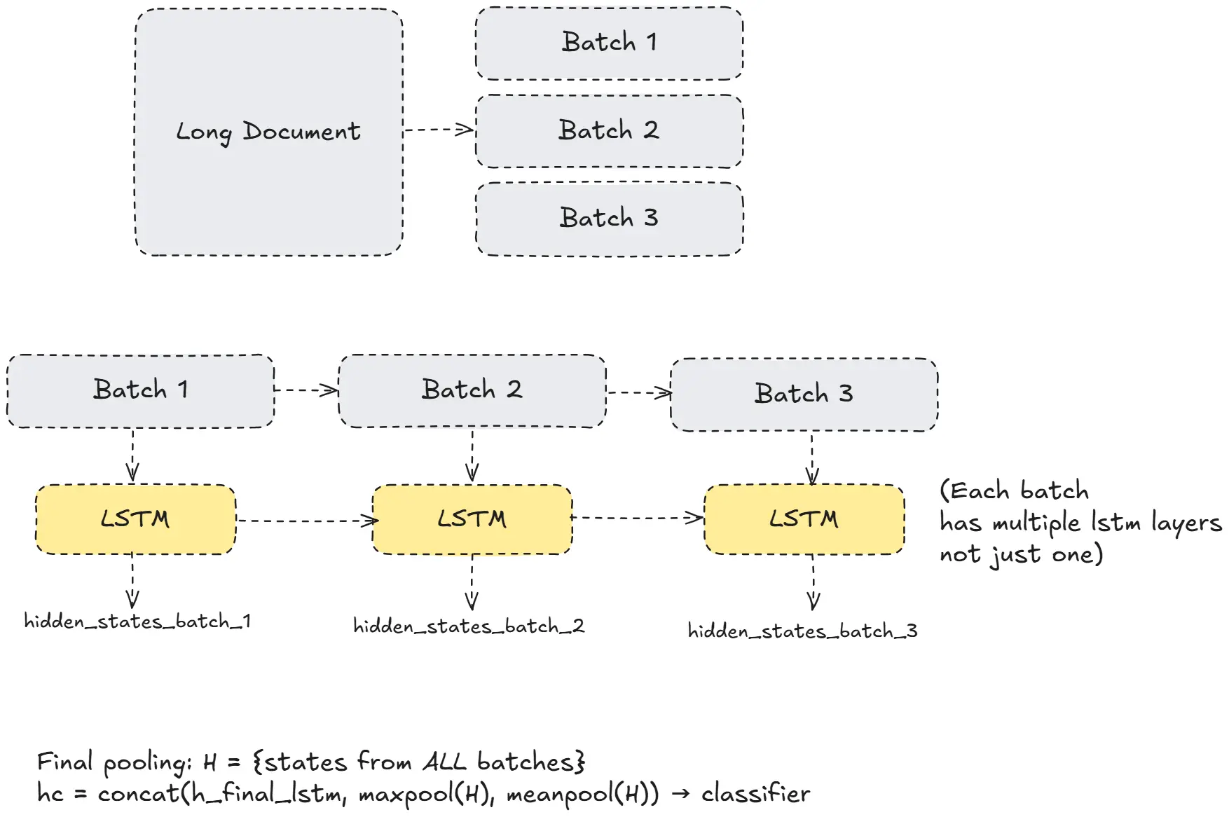
For handling long documents, ULMFiT adapts backpropagation through time by dividing documents into fixed-length batches while maintaining hidden state continuity between batches.
Revolutionary Results
ULMFiT’s results were unprecedented for their time. On six text classification datasets, the method achieved 18-24% error reduction compared to state-of-the-art approaches. More impressively, with just 100 labeled examples, ULMFiT matched the performance of training from scratch with 10-100× more data.
This sample efficiency was the real game-changer. Suddenly, high-quality NLP became accessible to domains with limited labeled data, democratizing the field in ways that hadn’t been possible before.
ELMo: Embeddings from Language Models
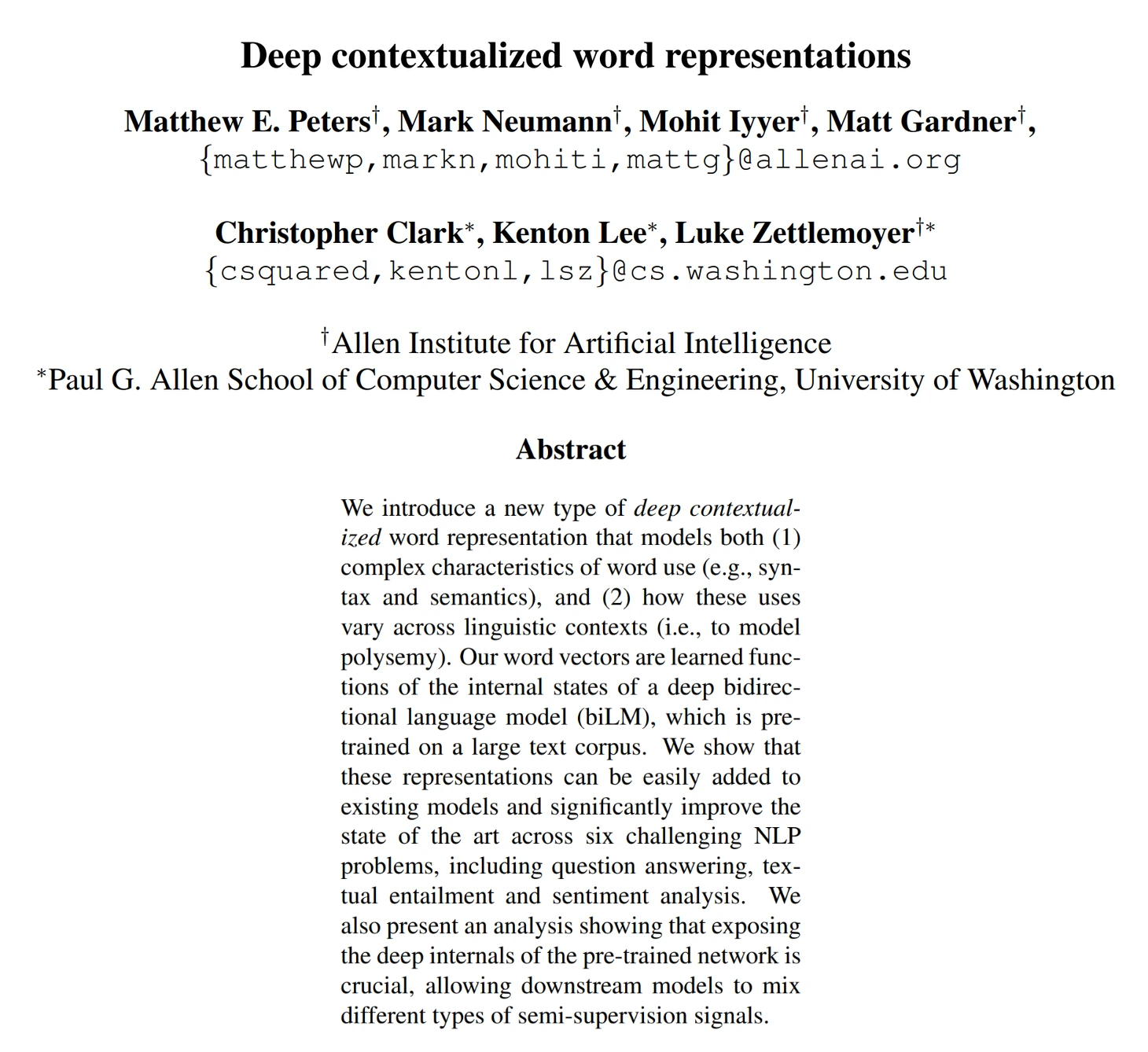
Link to paper: Deep contextualized word representations
Quick Summary
This paper introduces ELMo (Embeddings from Language Models), a new approach to creating word representations that capture both complex word characteristics (syntax and semantics) and how those characteristics change across different contexts (addressing polysemy). Unlike traditional word embeddings that assign a single vector per word, ELMo derives representations from a bidirectional language model (biLM) pre-trained on a large text corpus.
The key innovation is that ELMo representations are deep - they’re a function of all internal layers of the biLM, not just the final layer. The authors show that different layers capture different linguistic properties (lower layers capture syntax, higher layers capture semantics). By learning task-specific weightings of these layers, models can access both types of information simultaneously.
The authors demonstrate that adding ELMo to existing models significantly improves performance across six diverse NLP tasks, including question answering, textual entailment, sentiment analysis, and named entity recognition - achieving state-of-the-art results in all cases, with relative error reductions ranging from 6-20%.
Embeddings are a vital part of LLMs, because they determine the very understanding of tokens. Think of them as the language that allows machines to understand and work with human text. Just like how we might describe a person using various characteristics (height, age, personality), embeddings describe words using hundreds of numerical features that capture their meaning, relationships, and usage patterns.
Problem
Before ELMo, word embeddings had a major limitation: each word had only one representation regardless of context. The word “bank” would have the same vector whether you’re talking about a financial institution or the side of a river. This is called the polysemy problem - one word, multiple meanings, but only one embedding.
learning high quality representations can be challenging. They should ideally model both (1) complex characteristics of word use (e.g., syntax and semantics), and (2) how these uses vary across linguistic contexts (i.e., to model polysemy).
Solution
ELMo’s breakthrough was making embeddings contextual. Instead of giving “bank” the same representation everywhere, ELMo creates different representations based on the surrounding words. When “bank” appears near “loan” and “mortgage,” it gets a finance-related representation. When it appears near “river” and “water,” it gets a geography-related representation.
Our representations differ from traditional word type embeddings in that each token is assigned a representation that is a function of the entire input sentence. We use vectors derived from a bidirectional LSTM that is trained with a coupled language model (LM) objective on a large text corpus.
Before we start talking about ELMo we have to understand how word embeddings work and what they are. You can skip this section if you have an extensive understanding of the topic at hand
This book proved to be extremely helpful while writing this section.
Traditional Word Embeddings
Machines do not understand text but rather numbers. So researchers have come up with ways to represent words as numbers that still captures their complexity, semantics, meaning etc. Let’s go one by one.
One-Hot Vectors
One of the simplest solution is to create one hot encoding for each word.
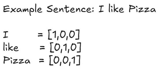
Here, every word has been assigned a unique vector and the length of our one-hot encoded vector would be equal to the size of $V$ ($|V| = 3$).
Note:
- In OHE words are independant of each other and hence do not capture any relationship between them
- OHE is computationally expensive as in reality the size of vocabulary can be in billions
Bag-of-Words (BOW)
Think of BOW as the most straightforward way to convert text into numbers - it’s like counting how many times each word appears in a document, completely ignoring the order.
BOW creates a document-term matrix where each row represents a document and each column represents a word from our vocabulary. Each cell contains the frequency of that word in that specific document.
# Simple BOW implementation
documents = ['this is the first document',
             'this document is the second document',
             'this is the third one',
             'is this the first document']

# Create vocabulary
vocab = []
for doc in documents:
    for word in doc.split():
        if word not in vocab:
            vocab.append(word)

# Create BOW matrix
bow_matrix = []
for doc in documents:
    word_count = [doc.split().count(word) for word in vocab]
    bow_matrix.append(word_count)

print("Vocab:", vocab)
print("BOW Matrix:", bow_matrix)

# Vocab:
# ['this', 'is', 'the', 'first', 'document', 'second', 'third', 'one']

#BOW Matrix:
# [[1, 1, 1, 1, 1, 0, 0, 0],
#  [1, 1, 1, 0, 2, 1, 0, 0],
#  [1, 1, 1, 0, 0, 0, 1, 1],
#  [1, 1, 1, 1, 1, 0, 0, 0]]
The problem? BOW treats “The cat sat on the mat” and “The mat sat on the cat” as identical because it only cares about word counts, not context or order. Plus, common words like “the” and “is” get the same weight as meaningful words.
Co-occurrence Matrix
Instead of just counting words in documents, what if we count how often words appear together? That’s exactly what co-occurrence matrices do.
A co-occurrence matrix shows how frequently word pairs appear within a defined window (like within the same sentence). If “learning” and “machine” often appear together, they’ll have a high co-occurrence score.
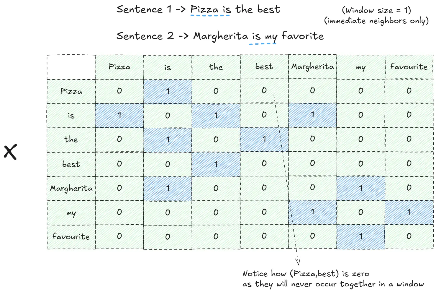
The mathematical representation: For words $w_i$ and $w_j$, the co-occurrence count $C_{ij}$ represents how many times they appear together within a context window.
\[C_{ij} = \sum_{k=1}^{N} \mathbb{I}(w_i, w_j \text{ co-occur in context } k)\]Where $\mathbb{I}$ is an indicator function and $N$ is the total number of contexts.
# Simple co-occurrence matrix
def build_cooccurrence_matrix(documents, window_size=1):
    # Flatten all documents into one list
    all_words = []
    for doc in documents:
        all_words.extend(doc.split())

    # Create vocabulary
    vocab = list(set(all_words))
    vocab_size = len(vocab)

    # Initialize matrix
    cooc_matrix = [[0 for _ in range(vocab_size)] for _ in range(vocab_size)]

    # Count co-occurrences
    for i in range(len(all_words)):
        target_word = all_words[i]
        target_idx = vocab.index(target_word)

        # Check words within window
        for j in range(max(0, i-window_size), min(len(all_words), i+window_size+1)):
            if i != j:
                context_word = all_words[j]
                context_idx = vocab.index(context_word)
                cooc_matrix[target_idx][context_idx] += 1

    return cooc_matrix, vocab
The beauty of co-occurrence matrices is that they capture some semantic relationships - words that often appear together likely have related meanings.
N-Gram
N-grams extend the BOW concept by considering sequences of $n$ consecutive words instead of individual words. This helps capture some word order and context.
- Unigrams (n=1): Individual words → [“this”, “is”, “the”, “first”]
- Bigrams (n=2): Word pairs → [“this is”, “is the”, “the first”]
- Trigrams (n=3): Word triplets → [“this is the”, “is the first”]
The mathematical formulation for n-gram probability: \(P(w_n|w_1, w_2, ..., w_{n-1}) \approx P(w_n|w_{n-k+1}, ..., w_{n-1})\)
def generate_ngrams(text, n):
    words = text.split()
    ngrams = []
    for i in range(len(words) - n + 1):
        ngram = ' '.join(words[i:i+n])
        ngrams.append(ngram)
    return ngrams
The trade-off? Higher n-values capture more context but create exponentially more features and become computationally expensive.
TF-IDF (Term Frequency-Inverse Document Frequency)
TF-IDF is the smart cousin of BOW. It doesn’t just count words - it considers how important a word is to a specific document relative to the entire collection.
The intuition: Words that appear frequently in one document but rarely across all documents are more significant for that specific document.
\[\text{TF-IDF}(t,d) = \text{TF}(t,d) \times \text{IDF}(t)\]Where:
- $\text{TF}(t,d) = \frac{\text{count of term } t \text{ in document } d}{\text{total words in document } d}$
- $\text{IDF}(t) = \log\left(\frac{\text{total documents}}{\text{documents containing term } t}\right)$
import numpy as np
import pandas as pd

documents_name = ["Document-1", "Document-2", "Document-3", "Document-4"]

documents = ['this is the first document',
             'this document is the second document',
             'this is the third one',
             'is this the first document']

word_tokens = []

for document in documents:
    words = []
    for word in document.split(" "):
        words.append(word)
    word_tokens.append(words)

vocab = set()

for document in word_tokens:
    for word in document:
        vocab.add(word)

vocab = list(vocab)

TF = [[0 for j in range(len(vocab))] for i in range(len(word_tokens))]

for i, document in enumerate(word_tokens):
    for word in document:
        j = vocab.index(word)
        TF[i][j] += 1 / len(word_tokens[i])

idf = [0 for i in range(len(vocab))]
D = len(word_tokens)

for j, word_vocab in enumerate(vocab):
    df = 0
    for document in word_tokens:
        for word in document:
            if word_vocab == word:
                df += 1
                break
    idf[j] = np.log(D/df)

TFIDF = [[0 for j in range(len(vocab))] for i in range(len(word_tokens))]

for i in range(len(word_tokens)):
    for j in range(len(vocab)):
        TFIDF[i][j] = TF[i][j] * idf[j]

data = pd.DataFrame(TFIDF, columns=vocab, index=documents_name).round(3)
data
Code taken from here
if we calculate tf-idf of the same example as before we get an output like below
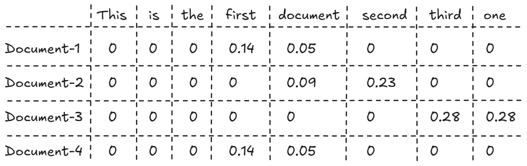
Notice how common words like “this”, “is”, “the” get lower TF-IDF scores because they appear in most documents, while specific words like “second” or “third” get higher scores.
The Limitation of Traditional Embeddings
All these methods share a fundamental flaw: they assign the same representation to a word regardless of context. The word “bank” gets the same vector whether we’re talking about a river bank or a financial institution. This is where contextual embeddings like ELMo come to the rescue.
Static Word Embeddings
Word2Vec
The following are excellect sources to understand Word2Vec in a deeper level. Consider going through them
Intuition
We are going to start with the old and cheesy explanation of Word2Vec. Talking about similarity of vector representation in space. (If you do not understand what I am talking about, Most explanations of Word2Vec use the explanation I am about to give. Fret not, for we will dive deeper too!)
I absolutely love cheese. And I have scale in which I measure how cheesy a piece of cheese is.
Anytime I find a new cheese, I taste it and put it on my scale. I use this scale to choose which cheese to eat based on my mood.
But one day I ran into a cheese (yellow cheese) which had the same cheesiness as the white cheese. Now how do I differentiate between the two? well cheese has many other properties (or features from the ML perspective). Like protein!!
I can add that as another axis and I can use that as another metric to choose the kind of cheese I want to eat.
This way of plotting cheese based on different properties provides with another amazing way. One day a friend of mine came and said he really liked red cheese, but I was out of red cheese :( because I love it too.
So I can just find the cheese which is most similar to it, using cosine similarity!!
That is essentially the idea of Word2Vec, We plot multiple words in an n dimensional space (I used 2 dimensional because I can plot it. I can’t plot a 7d space, I will love to meet you if you can tho!!!). And find similar words based on cosine similarity.
The cosine similarity between two vectors A and B is calculated as:
\[\cos(\theta) = \frac{A \cdot B}{||A|| ||B||} = \frac{\sum_{i=1}^{n} A_i B_i}{\sqrt{\sum_{i=1}^{n} A_i^2} \sqrt{\sum_{i=1}^{n} B_i^2}}\]This gives us a value between -1 and 1, where 1 means the vectors point in exactly the same direction (very similar), 0 means they’re perpendicular (unrelated), and -1 means they point in opposite directions (very different).
There is a popular example that shows the distance between king and woman is same as the distance between man and woman. This essentially shows that both the pair of words share very similar ideas with only a few differences (maybe in royalty).
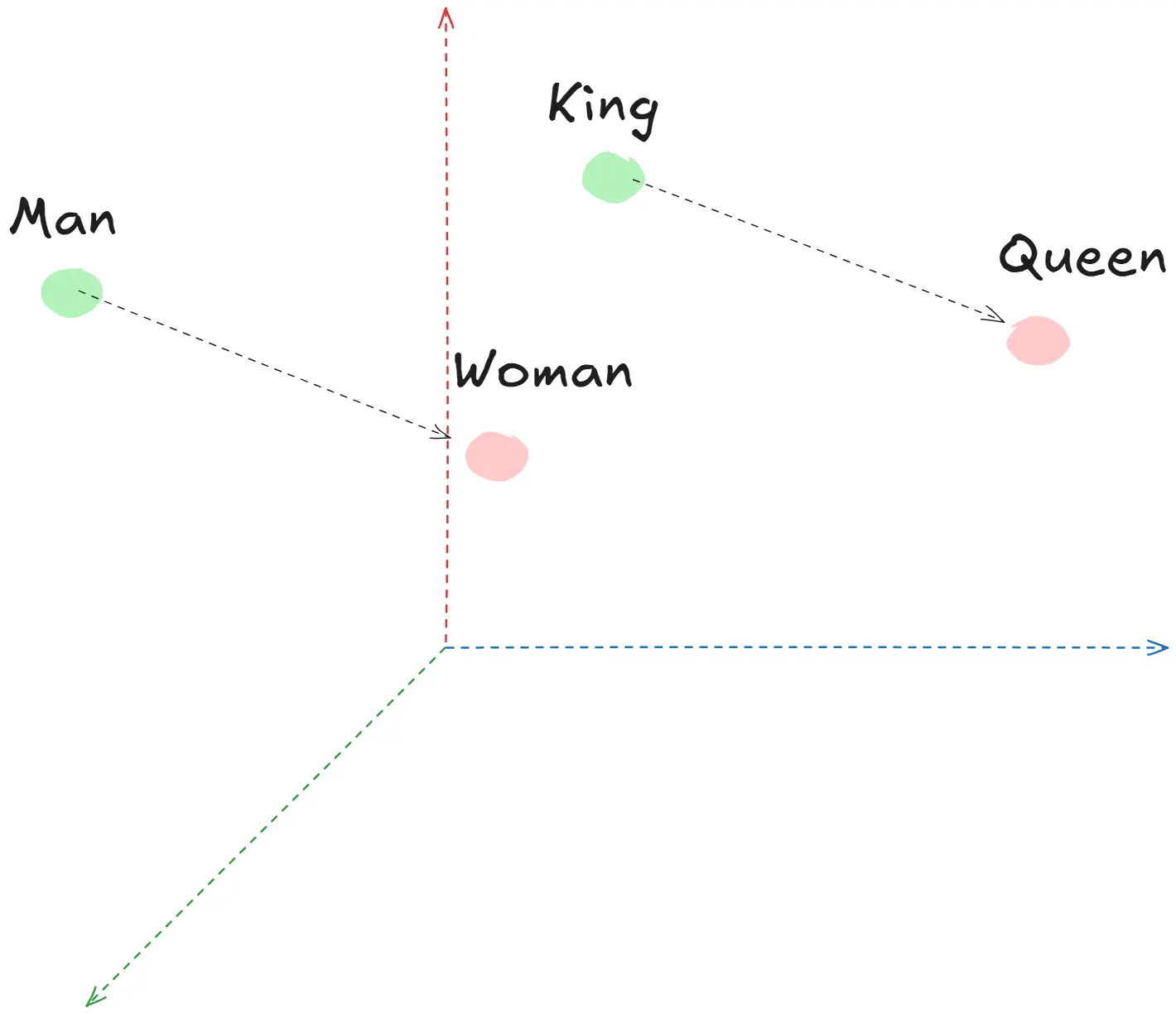
In reality Word2Vec looks something more like the below image (ouch!!).
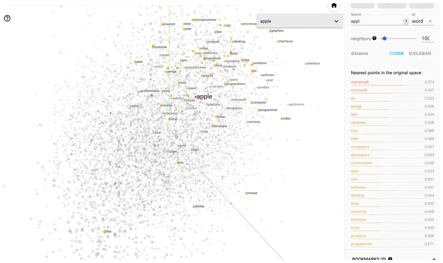 Image taken from Embedding Projector
Skip gram model
Now that we understand the idea behind Word2Vec, it’s time to understand how it is implemented. I will be skipping Continous Bag of words, an idea introduced in the original paper as it is not essential in my opinion. You can read more about it in the sources I have provided.
| Skip gram in 1 sentence -> Given a word, find it’s nearby words (context words). |
| CBOW in 1 sentence -> Given context words, find the target word. |
One of the many beautiful thing about NLP is, you can create a labelled dataset using an unlabelled dataset. Our objective is to build a model that finds words nearby a target word.
Let us understand how the training dataset is created using a sample sentence. We first define a window (here it’s 2), we have our target word with the relevant context words around it.
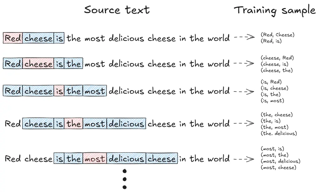
Now that we have our training data, let us understand how the model itself is constructed. Remember how we talked about cheesiness as a feature for our cheese, then protein, well both of them can be described as their own individual neuron. So in the example below we have an embedding model with 300 as it’s dimension (In modern embedding model when you talk about dimensions, it is essentially talking about how many features can be used to describe one particular token, as a rule of thumb higher the dimension, more complex is it’s representation)
So for any given word, we can create a one hot encoding, then pass it through our embedding model. Which is then passed to the final Softmax layer which gives the probability of all the words which are likely to be a context word.
I have a question for you, What is the difference between nn.Embedding and nn.Sequential?
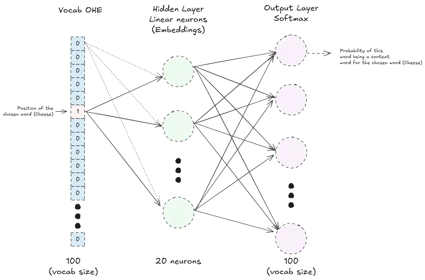
One thing I found interesting was, we talk about “Embedding Matrix” but the above image describes a typical neural network model, what is going on over here?
Well if we look below, it becomes much easier to understand. The word vector represents the OHE encoding of the chosen work.
Each row of the embedding matrix represents the weights of every word in that neuron. So when we do a matrix multiplication, we get the weight for that word from different neurons.
It’s easier to visualize as different embedding vectors for each token of a fixed dimension.
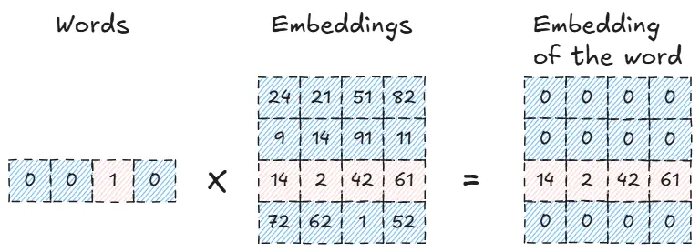
Now we just run a training loop and voila, the hidden layer, is our embedding matrix. But we have a problem. As this was an example we used a vocabulary of a 100 words, but in reality the vocabulary is 100x times larger. And calculating softmax of so many tokens is a very expensive operation.
imagine a vocabulary of 10,000 tokens (quite small from modern vocabs) with 500 dimensional embedding model. That’s 5 million training parameter!!!
There are a few solutions proposed by the researchers to overcome this problem. Interestingly the original paper only mentions Hierarical Softmax, but the code shared by researches talks about sub-sampling and Negative Sampling. So let’s talk about all three!
[UPDATE] I later found out that they introduced these ideas in there follow up paper here. (Have a look at the authors… it is something haha)
This blog covered the mentioned topics quite well and I have taken inspiration from it while writing this section.
Sub-Sampling
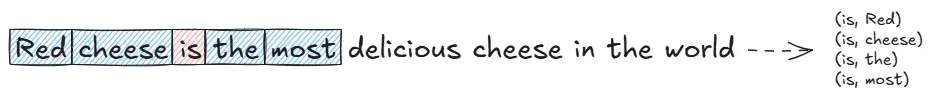
If we look at one particular example from our dataset generation step, particularly the 3rd line. We will see that is is a word that must be quite common in sentences. And hence we can expect to run into many pairs of is, ...
To fix this problem, the authors introduced a sampling rate.
\[P(w_i) = 1 - \sqrt{t/f(w_i)}\]Where $f(w_i)$ is the frequency of the word and $t$ is a chosen threshold.
Negative Sampling (better for frequent words, better with low dimensional vectors)
The idea is quite interesting, If we go back to the example that we started with. I.e training on a vocab of 100 words. Our main problem was that it was very expensive to calculate the softmax of so many tokens.
So what if instead of training on all the tokens, we took a small subset of the negative samples. I.e tokens which are not related to our target word, and take a bunch of context words. And train it using logistic regression. In other words, tell if two words are neighbours or not.
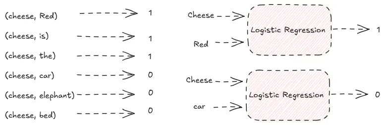
This greatly simplifies training, and reduces the cost significantly too. One interesting thing to note is the authors used a unigram distribution to pull the negative samples out of.
If you wish to learn more about negative sampling consider reading this.
I find “why this even works” more interesting than the fact that it works (And this produces better results than our original method). It’s actual name is noise contrastive estimation and the way I imagine it is, we are pulling similar words together while pushing dissimilar words away. Now if we pushed all of the dissimilar words away as we were doing we inevitably pushed away similar words for different pairs too.
Consider reading about contrastive loss. (This is a good medium article on the topic, Consider looking at the author of contrastive loss too… it’s somehting haha)
Hierarical Softmax (better for infrequent words)
Let’s start with an example, because that really drives the idea home.
“I can have pizza every day”
If we used the standard softmax to calculate the probability of “pizza” given some context, we would do something like:
\[P(pizza|context) = \frac{e^{v'_{pizza} \cdot h}}{\sum_{w \in V} e^{v'_w \cdot h}}\]Where $h$ is the hidden layer output (context vector) and $v’_w$ are the output embeddings.
But Hierarchical Softmax constructs a binary tree and we get a structure like below:
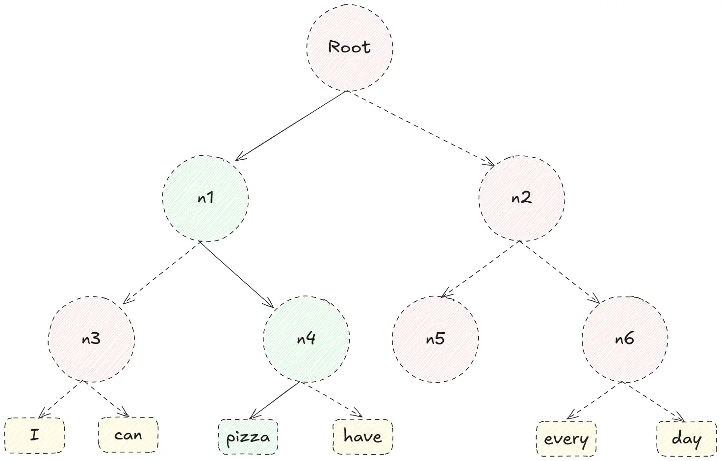
Understanding how the binary tree is constructed is beyond the scope of this article, but if you understand how Huffman Encoding works, that is one way of creating the tree. More frequent words get shorter paths, less frequent words get longer paths.
The equation then becomes:
\[P(pizza|context) = \sigma(v'_{root} \cdot h) \times \sigma(-v'_{n_1} \cdot h) \times \sigma(v'_{n_4} \cdot h)\]Where:
- $\sigma(x) = \frac{1}{1 + e^{-x}}$ is the sigmoid function
- $v’_{n_i}$ are the learned vectors for internal nodes
- The negative sign appears when we take the left branch at a node
This reduces the computation from $O(|V|)$ to $O(\log|V|)$, where $V$ is the size of the vocabulary.
If you wish to learn more about Hierarchical Softmax consider reading this blog.
GloVe
This blog helped me considerably while writing this section.
GloVe stands for Global Vectors for Word Representation, it is seemingly an improvement over Word2Vec as it considers global statistics over local statistics.
Well what does that mean? Put simply, we leverage the global co-occurrence matrix instead of using a local context window like we did in Word2Vec.
The main innovation behind GloVe is the idea that we only need to calculate the ratio of probability of the occurrence of two words to capture their semantic relation. This ratio-based approach helps filter out noise from non-discriminative words and highlights meaningful relationships.
First we create a co-occurrence matrix $X$ based on the available corpus. The notation $X_{ij}$ refers to number of times word j has appeared in the context of word i. We calculate the probability of a word j occurring given i as $P(j|i) = X_{ij}/X_i$, where $X_i$ is the sum of all co-occurrence counts for word i (i.e., $X_i = \sum_k X_{ik}$).
Let’s understand it with an example.
We created the co-occurrence matrix for two sentences “Pizza is the best” and “Margherita is my favorite” using a window size of 1 (immediate neighbors only).
Let’s calculate the probability of “Pizza” given “is” (this is from a very small corpus only to show how it is calculated, it is not reminiscent of the actual results).
From our matrix, “is” co-occurs with three words: “Pizza” (1 time), “the” (1 time), and “Margherita” (1 time). So the total count for “is” is 3.
\[P(\text{Pizza}|\text{is}) = \frac{X_{\text{is,Pizza}}}{X_{\text{is}}} = \frac{1}{3} = 0.33\]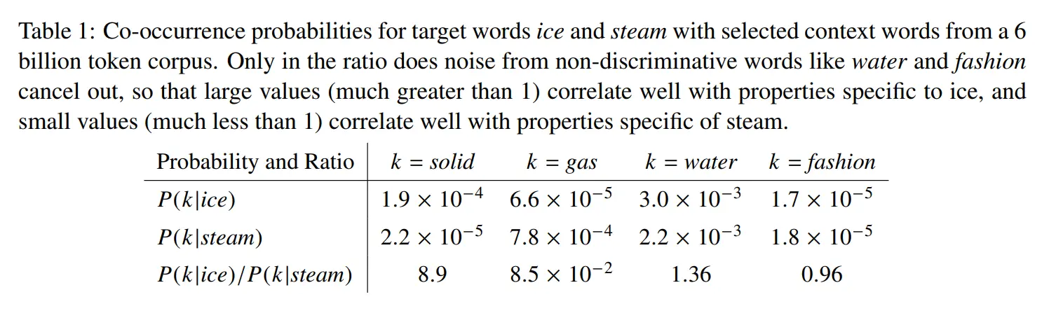 Image taken from the original paper
If we look at the example provided by the authors from a real corpus, the power of ratios becomes clear. It is pretty intuitive that $P(solid|ice)$ will have a higher value than $P(solid|steam)$, because “solid” is more likely to appear in the context of “ice” than “steam”. Hence their ratio $P(solid|ice)/P(solid|steam) = 8.9$ has a large value, indicating “solid” is discriminative for “ice”.
For “gas”, we see the opposite: $P(gas|ice)/P(gas|steam) = 0.085$, a small ratio indicating “gas” is discriminative for “steam”.
Whereas for “water”, both ice and steam are likely to co-occur with it, so the ratio $P(water|ice)/P(water|steam) = 1.36$ is close to 1, indicating “water” doesn’t discriminate between ice and steam. More interesting is “fashion” with a ratio of 0.96 ≈ 1, because both ice and steam are unlikely to be related to fashion. This ratio-based approach elegantly filters out such neutral co-occurrences that don’t provide semantic information.
This insight - that ratios of co-occurrence probabilities capture semantic relationships better than raw probabilities - forms the mathematical foundation of GloVe’s log-bilinear regression model.
To understand more about the implementation and training details, consider reading the original paper and this article.
I have skipped a lot of the different parts, like training, eval, results etc. Because this is ultimately a section on ELMo and not GloVe. But the idea is fascinating enough to garner some time spent on it.
Contextual Word Embeddings
Embeddings from Language Models (ELMo)
We more or less now have a complete understanding of how different embedding models work, so it’s time to understand the model of the hour: ELMo.
There are two things we need to understand: how it’s trained and how it’s used.
Training is quite simple - we train a two-layer bi-directional LSTM on a Language Modeling task.
The Language Modeling task basically means: given all these words, what’s the most likely word that comes next? It is exactly how GPT-1 was trained, which we will be covering next.
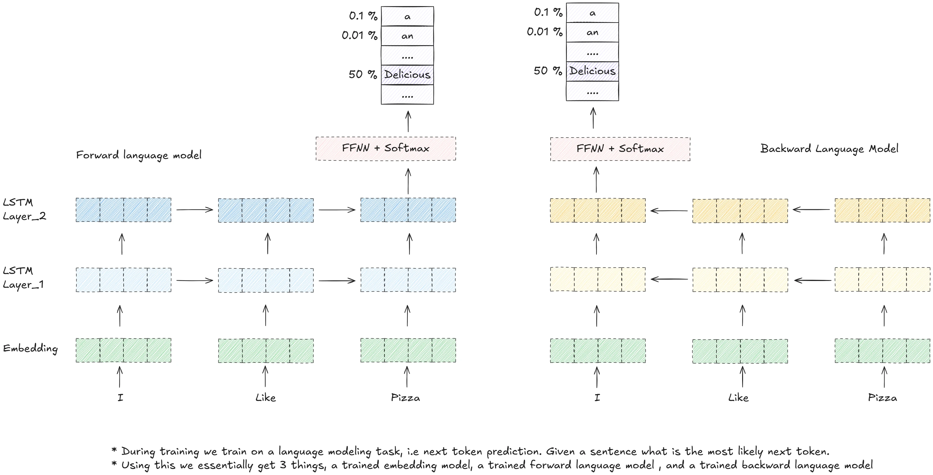 image inspired from this blog
Now I had a question while reading this: ELMo is an embedding model, right? But what we are doing is next token prediction here. How is it used with other NLP models then? If you have the same question, you are on the right track. It is quite an innovative solution in my opinion.
Let us first start with the very essence of any NLP task: We begin with a sentence, right? We can use this sentence, pass it to our trained ELMo model, and extract representations from different layers. The key insight is that we don’t just use the final layer - we combine representations from all layers (character embeddings + both LSTM layers) using learned weights.
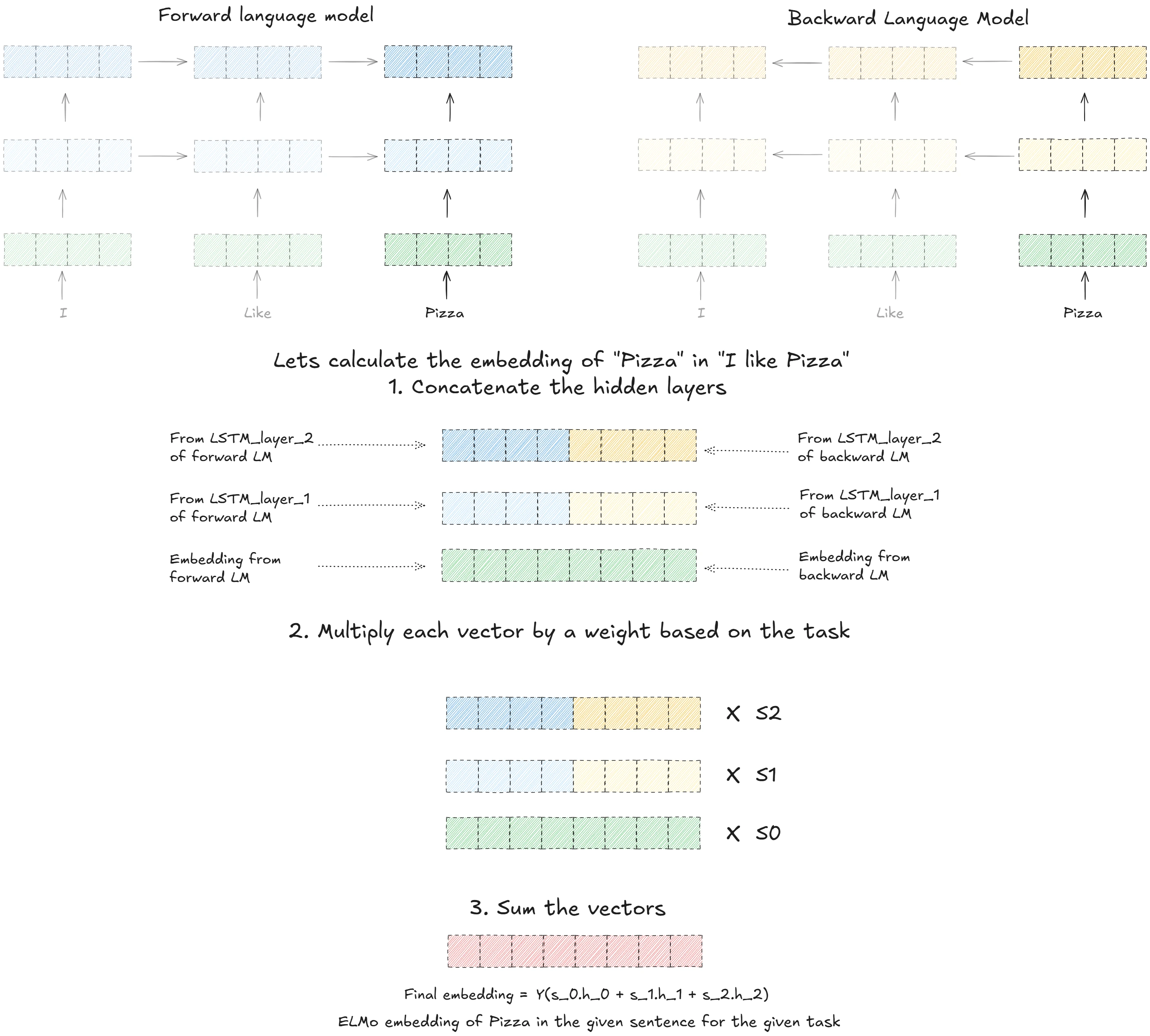
We can then give these combined embeddings to any other NLP model. Voila! This understanding will prove to be extremely useful as we move to bigger LLMs. While modern embedding models don’t use ELMo’s specific bidirectional LSTM approach, ELMo’s key innovation of contextual embeddings and the concept of using pre-trained language models for embeddings laid the groundwork for today’s transformer-based embedding models.
GPT-1
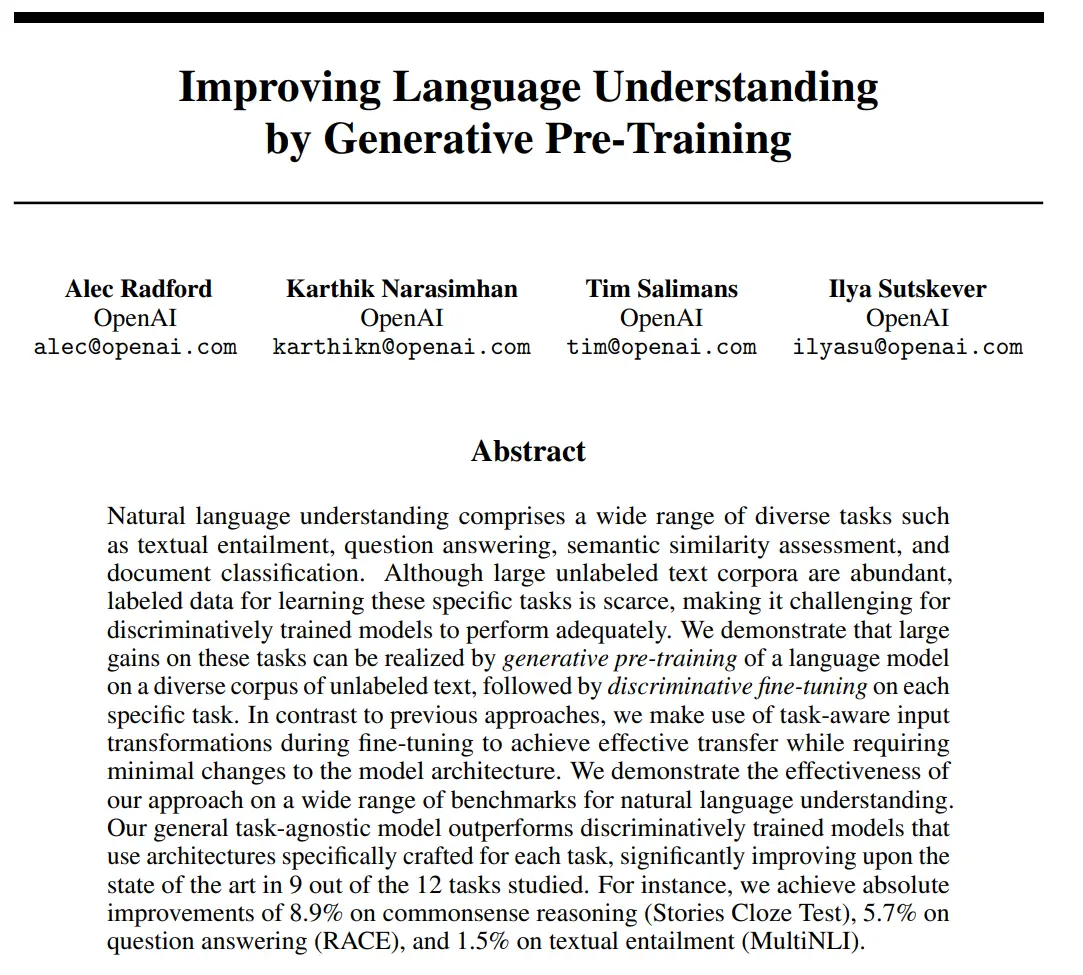
Link to paper: Improving Language Understanding by Generative Pre-Training , blog
Quick Summary
This seminal 2018 paper from OpenAI researchers (Radford, Narasimhan, Salimans, and Sutskever) introduces a powerful semi-supervised approach to natural language understanding that combines unsupervised pre-training with supervised fine-tuning.
The key innovation lies in training a large transformer-based language model on unlabeled text data, then leveraging the learned representations by fine-tuning this model on specific downstream tasks. This approach addresses a fundamental challenge in NLP: the scarcity of labeled data for various language understanding tasks.
The authors demonstrate that their method significantly outperforms task-specific architectures across 9 out of 12 NLP tasks, including natural language inference, question answering, semantic similarity, and text classification. Notable improvements include:
- 8.9% on commonsense reasoning (Stories Cloze Test)
- 5.7% on question answering (RACE)
- 1.5% on textual entailment (MultiNLI)
This approach minimizes task-specific architecture modifications by using “task-aware input transformations,” which convert structured inputs into a sequence format compatible with the pre-trained model.
This paper laid important groundwork for later transformer-based language models, demonstrating that generative pre-training on unlabeled data could significantly improve performance on downstream language understanding tasks.
GPT-1 was the moment when everything clicked. While ULMFiT showed that transfer learning could work in NLP and BERT demonstrated the power of bidirectional representations, GPT-1 proved that a simple, scalable approach just predicting the next word could create surprisingly capable language models. This paper didn’t just introduce a new model, it established the blueprint that lead to GPT-2, GPT-3, and the entire generative AI revolution.
Problem
The ability to learn effectively from raw text is crucial to alleviating the dependence on supervised learning in natural language processing (NLP). Most deep learning methods require substantial amounts of manually labeled data, which restricts their applicability in many domains that suffer from a dearth of annotated resources
Solution
In this paper, we explore a semi-supervised approach for language understanding tasks using a combination of unsupervised pre-training and supervised fine-tuning. Our goal is to learn a universal representation that transfers with little adaptation to a wide range of tasks. We assume access to a large corpus of unlabeled text and several datasets with manually annotated training examples (target tasks). Our setup does not require these target tasks to be in the same domain as the unlabeled corpus. We employ a two-stage training procedure. First, we use a Language Modeling objective on the unlabeled data to learn the initial parameters of a neural network model. Subsequently, we adapt these parameters to a target task using the corresponding supervised objective.
This was the beginning of the era we live in now. As funny as it may sound, I do not have a lot to add in this section. Because we have already talked about the majority things, the architecture and important concepts like attention in our transformers blog and the training method in our ULMFit section.
So let’s use this section, to talk about the terms we popularly associate with LLMs like Top k, Top p, Temperature, Sampling etc.
Also, since I wrote the transformers blog I have gained a deeper and better understanding of self-attention and masked attention, so we will spend a bit of time on that too.
I will be skipping most of the thing we have already talked about, but if you still wish to get a quick recap of everything you have learned so far about Language models. Consider reading this fabulous blog by Jay Alammar. (you may say that this blog is on gpt-2 and not gpt-1. Well truth be told there is not much difference in gpt, gpt-2 and gpt-3 beside their obvious scale.)
GPT ASAP
Generative Pre-trained Transformer is a decoder only auto-regressive model which was first pre-trained on a humongous amount of data using a Language Modeling method then fine-tuned on a much smaller supervised dataset to help solve specific tasks
That is a lot of ML jargon way of saying that, the authors took the transformer, got rid of the encoder, put up a lot of layers of decoder, trained it on lots of data, then fine tuned it for specific use cases.
Langaguage modeling is pretty straight forward, given a context, predict the next word. The amazing part is that it is unsupervised. We can create a dataset using any sentence/document/text data. We break it down to it’s individual tokens, then we create a dataset by shifting the tokens by 1.
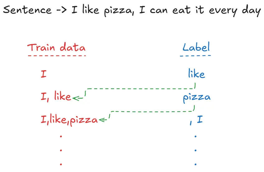
Model Specification
I took this excerpt directly from the paper as I cannot add anything else to it.
Model specifications Our model largely follows the original transformer work [62]. We trained a 12-layer decoder-only transformer with masked self-attention heads (768 dimensional states and 12 attention heads). For the position-wise feed-forward networks, we used 3072 dimensional inner states. We used the Adam optimization scheme [27] with a max learning rate of 2.5e-4. The learning rate was increased linearly from zero over the first 2000 updates and annealed to 0 using a cosine schedule. We train for 100 epochs on minibatches of 64 randomly sampled, contiguous sequences of 512 tokens. Since layernorm [2] is used extensively throughout the model, a simple weight initialization of N(0, 0.02) was sufficient. We used a bytepair encoding (BPE) vocabulary with 40,000 merges [53] and residual, embedding, and attention dropouts with a rate of 0.1 for regularization. We also employed a modified version of L2 regularization proposed in [37], with w = 0.01 on all non bias or gain weights. For the activation function, we used the Gaussian Error Linear Unit (GELU) [18]. We used learned position embeddings instead of the sinusoidal version proposed in the original work. We use the ftfy library2 to clean the raw text in BooksCorpus, standardize some punctuation and whitespace, and use the spaCy tokenizer.
Why does attention work
I am almost giddy writing this section because I find it astounding that this question never came to my mind. Why does attention even work, we all know it works. But why?
Even before I begin I NEED to mention all these amazing blogs that helped me build an intuition behind the idea
- Understanding the attention mechanism in sequence models by Jeremy Jordan
- Additive attention the paper that introduced the idea of attention
- Transformers from Scratch by Brandon Rohrer this is attention explained each matrix multiplication at a time
- Transformers from scratch by Peter Bloem a different approach but equally amazing
- Some Intuition on Attention and the Transformer by Eugene Yan if you are short on time, just read this.
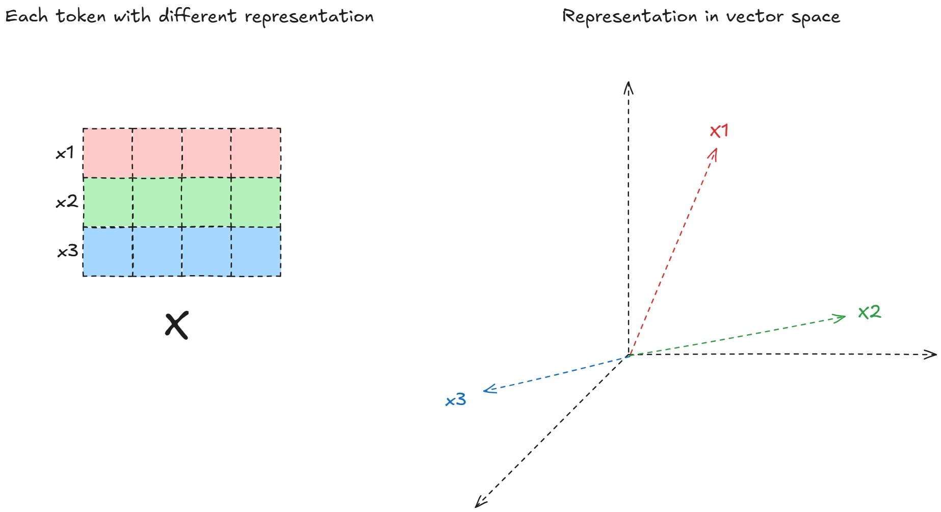
Let’s forget about Q,K,V for a moment and just focus on a single matrix X. Which contains different tokens (these tokens can be anything. Words, image patches, audio segments, anything that can be embedded and represented by numbers)
This matrix consists of vectors X1, X2, X2…. Xn That make up the matrix X
(X vectors are embedded so they occupy a specific place in space)
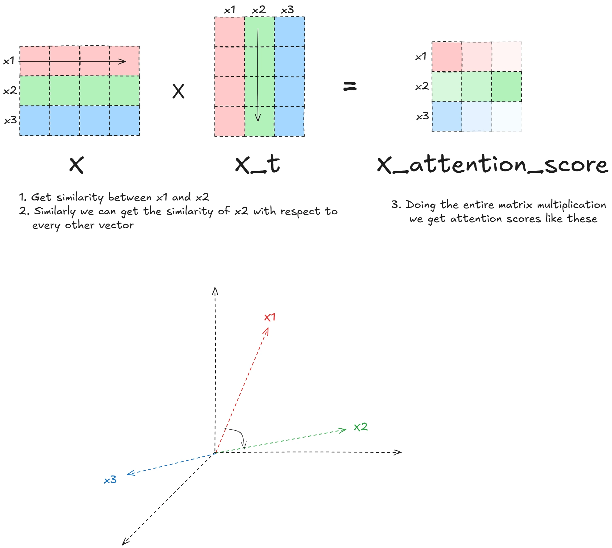
Now assume you want to see how close X1 is relative to every other word. What do you do? Take dot product, which gives us similarity scores between vectors - the higher the dot product, the more similar (or ‘closer’) the vectors are in the semantic space.
Now let’s say you want to see, how different vectors relate to X1, I.e How far is X2 from X1 (notice how we went from how far X1 is from X2, X3 and so on. To how far X2 is from X1).
Both of the above dot products will give us the same result. I.E how far each vector is relative to each other. This is ATTENTION. Distance between different words. We can think of like this.
In a sentence, “Steve is an amazing person, who loves Machine Learning”. After applying attention, a lot of words will basically get filtered out because we are not paying attention to them anymore
So the sentence becomes
“Steve … amazing …. Machine learning”
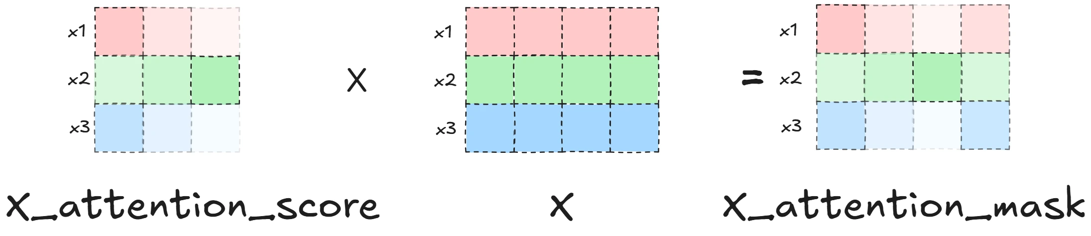
Now we need to apply these masks to something right, Hence we need to know the original sentence as well
So we multiply this mask with X. This gives us an attention mask over the original matrix.
We just calculated Self-attention. With 1 sentence. Without using the terms Q,K,V.
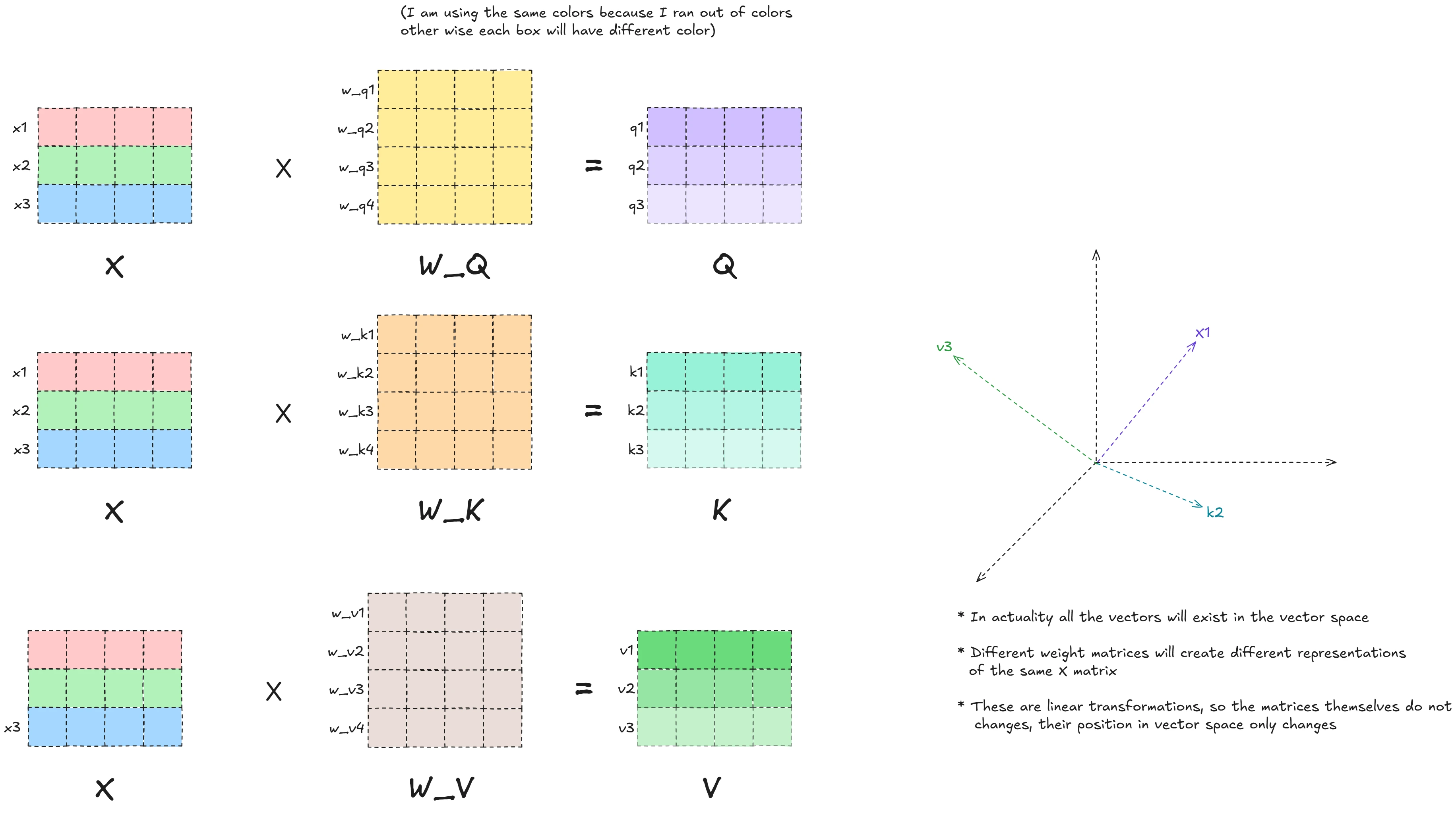
Now the question arises of W_q, W_k, W_v.
These are linear transformations, they are present to change the position of our X in the vector space.
But dot product gives us the similarity between different vectors in space, by changing representations. We are getting the similarity score from different angles.
This proves that attention works, because dot product is just giving us the similarity in space. What about “but which layer gives us what”
Think of it this way, lets assume our W matrices are all identity matrix. (so no transformation), Now when we do our attention scoring. If any token is more close to any other token it will get a very high score. This essentially gives us the attention of that pair. This will be represented in the first layer, the second layer will then calculate the attention of pairs (much like how CNNs work and are visualized. You start with small lines, then move on to more complex geometric figures)
Now by changing our W matrices in all different ways, we get different representation. And make pairs of different tokens stronger.
Masked Attention
Masked Attention is much like attention itself, but here we get rid of the bi-directional nature. The current token can only look at itself and the tokens before it.
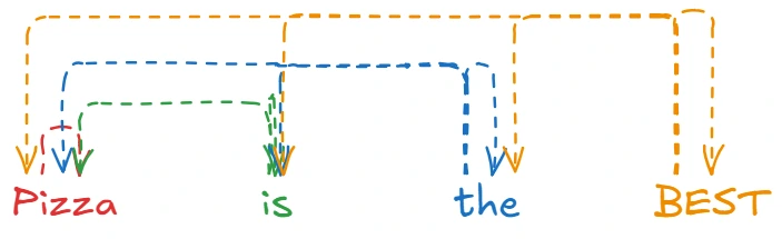
In a matrix representation is looks something like this, It is very vital. Because our inference is auto-regressive so if during training we can look at the future tokens we run into data leakage, the model would essentially be “cheating” by seeing the answer during training, making it unable to generate text properly during inference when it only has access to previous tokens.
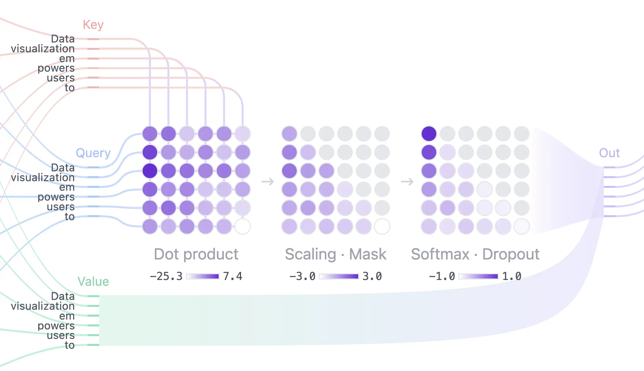 Image taken from this beautiful visualizer
The image shows how masked attention works in practice. First we calculate the attention score by multiplying Q and K, then a mask is applied to it. Each token (represented by the colored circles) can only attend to itself and the tokens that came before it. The connections show which tokens each position can “see”, notice how the connections always flow backwards or stay at the same position, never forward. This creates the triangular pattern you see in attention matrices, ensuring the model learns to predict based only on past context.
LLM Glossary
What this is -> A mathematical foundation for terms commonly used during LLM inference
What this is not -> A guide to deciding the best values for your use case
Temperature
\[P(token_i) = \frac{e^{logit_i/T}}{\sum_j e^{logit_j/T}}\]where T is temperature.
Temperature controls the randomness of token selection by scaling the logits before applying softmax. When T=1, we get the original distribution. As T approaches 0, the model becomes deterministic (always picks the highest probability token). Higher T values (>1) flatten the distribution, making the model more creative but potentially less coherent.
For example if Temperatur is 0, we will always get the same response from the model no matter how many times we run it, for Temperature = 1 we will get varied results.
Top K
\[P_{new}(token_i) = \frac{p_i}{\sum_{j=1}^k p_j}\]for $i \leq k$, and 0 otherwise
Top-k sampling restricts token selection to only the k most probable tokens, setting all other probabilities to zero before renormalization. If the original probabilities are $[p_1, p_2, …, p_n]$ sorted in descending order, top-k keeps only $[p_1, p_2, …, p_k]$ and renormalizes the tokens using the above formula. This prevents the model from selecting very unlikely tokens while maintaining some randomness.
For example,if the model earlier had 10 most likely options to choose from, by setting Top k=3 we are liminting those options to only 3 most likely options.
Top P (Nucleus Sampling)
\[\sum_{i=1}^k p_i \geq p\]Top-p sampling dynamically selects the smallest set of tokens whose cumulative probability exceeds threshold p. Given sorted probabilities $[p_1, p_2, …, p_n]$, we find the smallest k such that helps us clear the above criteria, then renormalize only these k tokens. Unlike top-k which uses a fixed number of tokens, top-p adapts to the confidence of the model - using fewer tokens when the model is confident and more when uncertain.
for example, if the model is fairly certain we will have the top token probabilities like [70%, 20%, 4%, 1% …] and if we set top p threshold as 93% we will make the model choose from the top 3 tokens only But if the model is uncertain and we get probabilities like [30%,29%,7%,5%,3%…] the model will have many tokens to choose from.
Sampling Methods
Sampling methods introduce controlled randomness by selecting tokens according to their probability distribution, often producing more diverse and human-like text at the cost of potential coherence.
\[token = \arg\max_i P(token_i)\]Greedy sampling always selects the token with highest probability. While deterministic and fast, this can lead to repetitive text and suboptimal sequences due to the exposure bias problem.
\[score(sequence) = \frac{1}{|sequence|^\alpha} \sum_{i=1}^{|sequence|} \log P(token_i|context_i)\]Where α is a length penalty to prevent bias toward shorter sequences.
Beam search maintains multiple candidate sequences simultaneously and explores the most promising ones. Instead of greedily picking the best token at each step, it keeps track of the top k sequences (beams) and expands each one.
Random sampling selects tokens according to their probability distribution without any constraints. While this can produce creative outputs, it often leads to incoherent text as low-probability tokens get selected too frequently.
Consider checking out the transformers documentation by HF.
Repetition Penalty
Repetition penalty reduces the probability of tokens that have already appeared in the generated sequence. The modified logit for a token that appeared n times is:
\[logit_{new} = \frac{logit_{original}}{penalty^n}\]if penalty > 1, which decreases the likelihood of selecting repeated tokens. This helps prevent the model from getting stuck in repetitive loops while maintaining natural language flow.
Frequency Penalty
Similar to repetition penalty but applies a linear reduction based on token frequency
\[logit_{new} = logit_{original} - \alpha \times count(token)\]where α is the penalty coefficient and count(token) is how many times the token appeared. This provides more nuanced control over repetition compared to the exponential scaling of repetition penalty.
Presence Penalty
A binary version of frequency penalty that applies a fixed penalty regardless of how many times a token appeared
\[logit_{new} = logit_{original} - \alpha\]if the token was seen before, unchanged otherwise. This encourages the model to use new vocabulary without heavily penalizing natural repetitions that occur in coherent text.
That wraps up our section on GPT, don’t worry as we move forward to the future years we will talk about how LLMs work with RL, How different architectures affect different things, talk about optimizers and so much more. For now I feel like these are the most we should keep for this year.
Sentencepiece
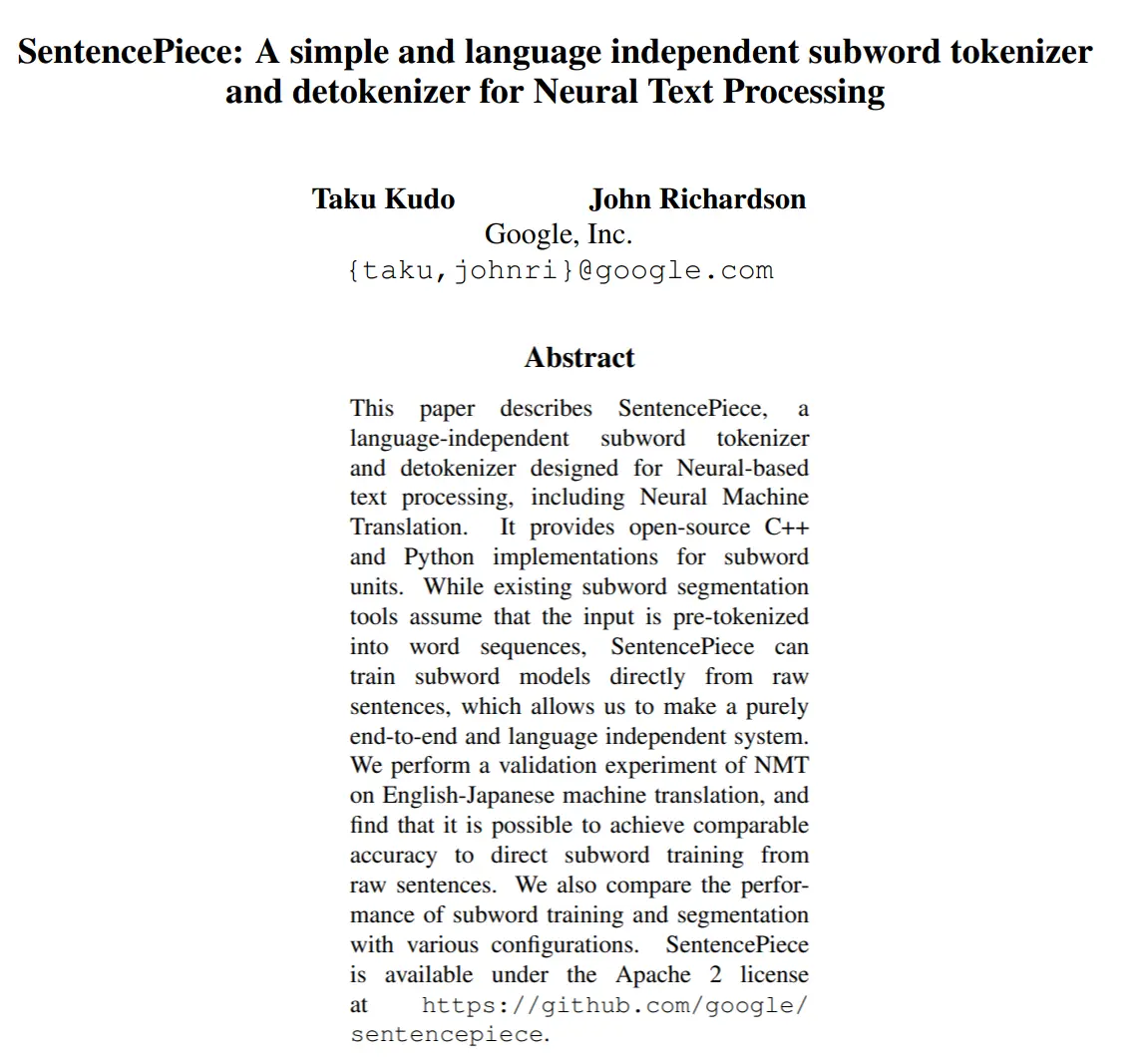
Link to the paper: SentencePiece: A simple and language independent subword tokenizer and detokenizer for Neural Text Processing
Quick Summary
This paper introduces SentencePiece, an open-source subword tokenizer and detokenizer designed specifically for neural text processing, including Neural Machine Translation (NMT). The key innovation of SentencePiece is that it can train subword models directly from raw sentences without requiring pre-tokenization, enabling truly end-to-end and language-independent text processing.
The authors highlight several important features:
- It implements two subword segmentation algorithms: byte-pair encoding (BPE) and unigram language model
- It provides lossless tokenization that preserves all information needed to reconstruct the original text
- The model is fully self-contained, ensuring reproducibility across implementations
- It offers efficient training and segmentation algorithms
- It includes library APIs for on-the-fly processing
They validate their approach through experiments on English-Japanese translation, showing comparable accuracy to systems that use pre-tokenization, while being significantly faster for non-segmented languages like Japanese.
Tokenization might seem like a boring preprocessing step, but it’s actually one of the most crucial components of any language model. Think of it as teaching a computer how to “read” - before a model can understand Shakespeare or debug your code, it needs to know how to break text into meaningful chunks. SentencePiece was a game-changer because it made this process truly language-agnostic.
Problem
Tough to make NMT language independent
Before SentencePiece, building multilingual NLP systems was a nightmare. Each language needed its own custom preprocessing pipeline - Japanese needed special word segmentation, Chinese required different tokenization rules, and languages like Thai had their own complexities. This meant you couldn’t easily train one model across multiple languages, severely limiting the scope and efficiency of NLP systems.
Solution
SentencePiece comprises four main components: Normalizer, Trainer, Encoder, and Decoder. Normalizer is a module to normalize semantically equivalent Unicode characters into canonical forms. Trainer trains the subword segmentation model from the normalized corpus. We specify a type of subword model as the parameter of Trainer. Encoder internally executes Normalizer to normalize the input text and tokenizes it into a subword sequence with the subword model trained by Trainer. Decoder converts the subword sequence into the normalized tex
The following articles helped me write this section
What are tokenizers?
As we have discussed earlier. Machines do not understand words, They understand numbers. Tokens are basically words represented as numbers that Language Models use to communicate. (You will see why this is an oversimplification in a minute?)
Why call them tokens if they are just words?
Taking back what I said, they aren’t exactly words. Let us understand why.
Word Level Tokenization
Let’s start with a simple sentence and tokenize (converting words in a document to token) it.
Example: “I love machine learning”
Tokens: [“I”, “love”, “machine”, “learning”]
Token IDs: [1, 234, 5678, 9012]
Now imagine instead of a sentence, it was a page, or a whole book. It will contain thousands if not hundreds of thousands of unique words. There are languages which have more than a million unique words. It will be unfeasible to tokenize each word.
Also what if we run into a word we have never seen during training. That will break our model, to overcome this, we can use something called Character Level Tokenization.
Character Level Tokenization
Let’s again start with the same sentence
Example: “I love machine learning”
Tokens: [“I”, “ “, “l”, “o”, “v”, “e”, “ “, “m”, “a”, “c”, “h”, “i”, “n”, “e”, “ “, “l”, “e”, “a”, “r”, “n”, “i”, “n”, “g”]
Token IDs: [1, 2, 12, 15, 22, 5, 2, 13, 1, 3, 8, 9, 14, 5, 2, 12, 5, 1, 18, 14, 9, 14, 7]
This fixes our problem of a huge vocabulary, but we run into another issue. Characters by themselves do not hold any meaning. This removes any semantic relation.
There have been innovations made to fix these problems, let’s look into them one by one.
Subword Tokenization
The idea is quite simple, In our previous word level tokenization. Fun, Funny, Funniest ,and other variations of the word Fun will be treated as different tokens. So in sub-word tokenization. We break down the words, something like Fun + niest.
The reason being in english we add a lot of different pre-fixes (Like un to funny that makes it unfunny) and suffixes (Like niest to Fun to get Funniest). The techniques of forming these subwords varies from different techniques to different techniques. Let’s explore them
Byte-pair encoding
This blog helped me immensely with this section.
Byte-pair encoding (BPE) was introduced in Neural Machine Translation of Rare Words with Subword Units (Sennrich et al., 2015). This is the encoding method the famous tiktoken tokenizer of OpenAI uses.
It essentially follows two steps, the pretokenization then merging. Let’s understand each.
In the pretokenization step, we determine the set of unique words in the training data along with their frequency. Using this unique set, BPE breaks the words down into it’s individual characters, which are then merged to form the final vocabulary. Let’s understand it with an example.
Suppose after the pre-tokenization step, we have the following words with their frequencies that we got from the training data
("hug", 10), ("pug", 5), ("pun", 12), ("bun", 4), ("hugs", 5)
Consequently, the base vocabulary is ["b", "g", "h", "n", "p", "s", "u"]. Splitting all words into characters of the base vocabulary, we get:
("h" "u" "g", 10), ("p" "u" "g", 5), ("p" "u" "n", 12), ("b" "u" "n", 4), ("h" "u" "g" "s", 5)
BPE then counts the character pair with the high frequencies and then pairs them up. Like here it will first pair up u and g as they occur the most together (10 times in hug, 5 times in pug and 5 more times in hugs. Totalling 20 times). This pair ug is then added to the vocabulary.
("h" "ug", 10), ("p" "ug", 5), ("p" "u" "n", 12), ("b" "u" "n", 4), ("h" "ug" "s", 5)
Then we identify the next most frequent pair, that will be u and n that occur 16 times together. Then the next most frequent pair interestingly is h with ug which occur together 15 times. (This teaches an important lesson, we do not only consider characters or symbols while pairing them up. But the frequency pairs that exist in the vocabulary).
Now our entire vocabulary looks something like this ["b", "g", "h", "n", "p", "s", "u", "ug", "un", "hug"] and our set of unique words
("hug", 10), ("p" "ug", 5), ("p" "un", 12), ("b" "un", 4), ("hug" "s", 5)
Assuming we stop our merging at this point. Our new vocabulary will be used to tokenize new words (Unless they were not present in our training data). For example, "bug" will be tokenized to ["b", "ug"] but “mug” would be tokenized as ["<unk>", "ug"] since the symbol "m" is not in the base vocabulary.
In general, single letters such as “m” are not replaced by the “
Using BPE the vocab size is the base vocabulary size + the number of merges, which is a hyperparameter we can choose. For instance GPT has a vocabulary size of 40,478 since they have 478 base characters and chose to stop training after 40,000 merges.
Wordpiece
Wordpiece is very similar to our BPE algorithm. It starts with the same idea of pre-tokenization followed by merging. It differs in the way it merges - instead of following the highest frequency, it merges based on a scoring system that considers how valuable each merge is.
The key difference is in how pairs are selected for merging:
WordPiece doesn’t just pick the most frequent pair like BPE does. Instead, it calculates a score for each pair by dividing how often the pair appears together by how often each part appears separately. This means it prefers to merge pairs where the individual parts are rare on their own, but common when together. This approach ensures that merges actually improve the tokenization rather than just combining frequent but unrelated pieces.
\[score = \frac{freq\_of\_pair}{freq\_of\_first\_element \times freq\_of\_second\_element}\]HF also has a short course on LLMs where they talk about wordpiece pretty well.
Taking an excerpt from the said course explains it well
By dividing the frequency of the pair by the product of the frequencies of each of its parts, the algorithm prioritizes the merging of pairs where the individual parts are less frequent in the vocabulary. For instance, it won’t necessarily merge (“un”, “##able”) even if that pair occurs very frequently in the vocabulary, because the two pairs “un” and “##able” will likely each appear in a lot of other words and have a high frequency. In contrast, a pair like (“hu”, “##gging”) will probably be merged faster (assuming the word “hugging” appears often in the vocabulary) since “hu” and “##gging” are likely to be less frequent individually.
If you are interested, I will recommend reading this blog by google which talks about Wordpiece more in depth.
Unigram
The same course talks about Unigram as well.
Unigram is quite different from our previously discussed tokenization methods like BPE and WordPiece. Instead of expanding the vocabulary, it starts with a big vocabulary and gradually trims down irrelevant tokens.
At each step of training, the Unigram model computes the loss over the entire corpus. Then, for each token it calculates how much the loss will increase if the token is removed, and removes the ones which increase the loss the least.
Note that we never remove the base characters, to make sure any word can be tokenized.
Using the same example as above we start with a sample corpus
("hug", 10), ("pug", 5), ("pun", 12), ("bun", 4), ("hugs", 5)
We calculate the frequencies of all the subwords as below
("h", 15) ("u", 36) ("g", 20) ("hu", 15) ("ug", 20) ("p", 17) ("pu", 17) ("n", 16)
("un", 16) ("b", 4) ("bu", 4) ("s", 5) ("hug", 15) ("gs", 5) ("ugs", 5)
To tokenize a given word, we look at all possible subwords and calculate their probabilities. All the tokens are considered independent of each other so we can just multiply all sub-tokens as below
For the word hug, by tokenizing it as h,u, and g
\(P(h) \times P(u) \times P(g)\) \(\frac{15}{210} \times \frac{36}{210} \times \frac{20}{210} = 0.000389\)
It is also tokenized as hu, g and h, ug, and hug. The scores are
["h", "u", "g"] = 0.000389
["hu", "g"] = (15/210) × (20/210) = 0.0095
["h", "ug"] = (15/210) × (20/210) = 0.0095
["hug"] = 15/210 = 0.071
Hence hug will be tokenized as [“hug”] as it has the highest probability.
In practice this iterative process is not used, but rather Viterbi algorithm is used to find the subword tokenization with the maximum probability.
Using this same method a score is calculated for all the words, as below
"hug": ["hug"] (score 0.071428)
"pug": ["pu", "g"] (score 0.007710)
"pun": ["pu", "n"] (score 0.006168)
"bun": ["bu", "n"] (score 0.001451)
"hugs": ["hug", "s"] (score 0.001701)
We want to calculate the negative log likelihood of the whole corpus and that becomes
freq("hug") × (-log(P("hug"))) + freq("pug") × (-log(P("pug"))) + freq("pun") × (-log(P("pun"))) + freq("bun") × (-log(P("bun"))) + freq("hugs") × (-log(P("hugs")))
10 × (-log(0.071428)) + 5 × (-log(0.007710)) + 12 × (-log(0.006168)) + 4 × (-log(0.001451)) + 5 × (-log(0.001701)) = 169.8
Now each token is removed to see how that affects the overall loss as below
Removing token “pu”: Loss change = 0 (since “pug” can use [“p”, “ug”] with same score) Removing token “hug”: Loss increases by 23.5 (forces less optimal tokenizations)
Tokens with the smallest loss increase are removed first until the desired vocabulary size is reached.
SentencePiece
This is a fabulous blog on the topic, it explains everything along with the implementation code. Consider checking it out.
This sub-section will be the shortest even though this section is about sentencepiece, you know why? well because sentencepiece is not a tokenizer at all, it’s a pre-tokenization algorithm used in conjunction with unigram or BPE.
All tokenization methods talked about so far have the same problem, they assume that the input text uses spaces to separate words. However, not all languages use spaces to separate words. One possible solution is to use language specific pre-tokenizers, e.g. XLM uses a specific Chinese, Japanese, and Thai pre-tokenizer. To solve this problem more generally, SentencePiece treats the input as a raw input stream, thus including the space in the set of characters to use. It then uses the BPE or unigram algorithm to construct the appropriate vocabulary.
Decoding with SentencePiece is very easy since all tokens can just be concatenated and “▁” is replaced by a space.
All transformers models in the library that use SentencePiece use it in combination with unigram. Examples of models using SentencePiece are ALBERT, XLNet, LLama2, etc.
Well that is all there is to know about SentencePiece really, if you want to know how it is implemented you can check out the blog I mentioned above.
BERT
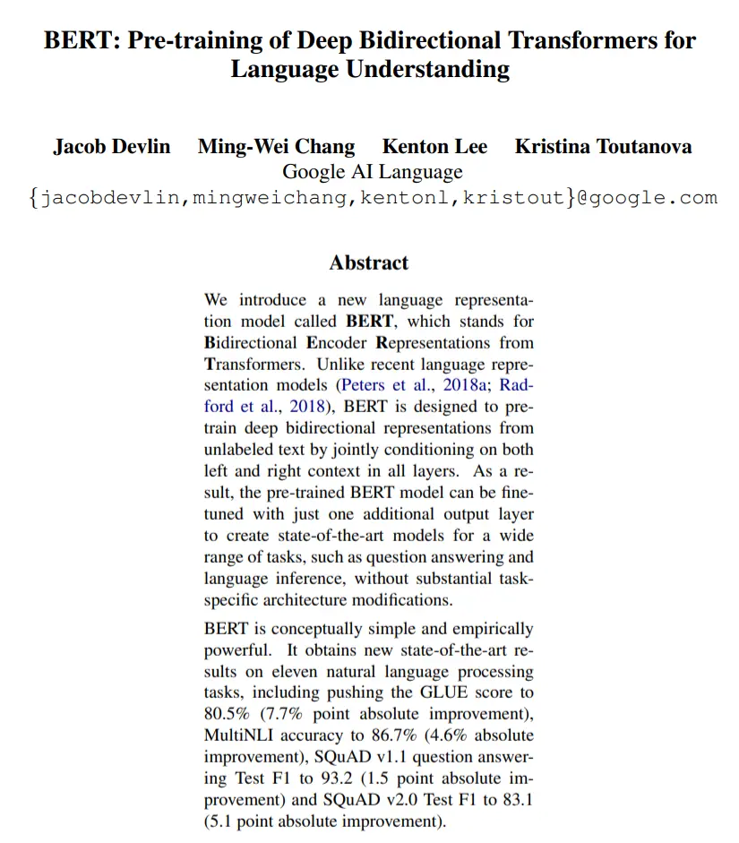
Link to paper: BERT: Pre-training of Deep Bidirectional Transformers for Language Understanding
Quick Summary
This paper introduces BERT (Bidirectional Encoder Representations from Transformers), a groundbreaking language representation model that significantly advanced the state of natural language processing in 2018. The key innovation of BERT is its ability to pre-train deep bidirectional representations from unlabeled text, unlike previous models that were limited to unidirectional contexts (either left-to-right or right-to-left).
BERT employs two novel pre-training tasks:
- Masked Language Model (MLM): Randomly masks some percentage of input tokens and predicts those masked tokens
- Next Sentence Prediction (NSP): Predicts whether two sentences follow each other in original text
These pre-training objectives allow BERT to create context-aware representations that capture information from both left and right contexts. After pre-training on large text corpora (BookCorpus and Wikipedia), BERT can be fine-tuned with just one additional output layer to create state-of-the-art models for a wide range of NLP tasks without task-specific architecture modifications.
The paper demonstrated significant improvements over previous methods on eleven NLP tasks, including the GLUE benchmark, SQuAD, and SWAG datasets.
These two blogs helped me immensely with this section:
This paper wasn’t trying to find a problem then solve it per se. It is more of an innovation, taking an excerpt from the paper.
BERT is designed to pretrain deep bidirectional representations from unlabeled text by jointly conditioning on both left and right context in all layers. As a result, the pre-trained BERT model can be finetuned with just one additional output layer to create state-of-the-art models for a wide range of tasks, such as question answering and language inference
Problem
Previous language models like GPT-1 and ELMo had a fundamental limitation: they could only look in one direction. GPT-1 used masked attention (only seeing previous tokens), while ELMo concatenated separate left-to-right and right-to-left models. But human language understanding is inherently bidirectional - to understand “The animal didn’t cross the street because it was too [tired/wide],” you need context from both sides to know whether “it” refers to the animal or the street.
Solution
BERT solved this by using the encoder portion of the Transformer architecture, which allows true bidirectional attention. Instead of predicting the next word (like GPT), BERT learns by predicting masked words using context from both directions simultaneously.
All the papers I have mentioned in this blog are great, but the BERT paper is particularly awesome. It stands out even today, and the sheer amount of innovations from one paper is astounding. I implore you to check it out.
Let’s first answer the question what is BERT?
BERT stands for Bi-directional Encoder Representation from Transformers. That’s a mounthful, the name aside. It is quite simple, Remember our Transformers, Well this is essentially that but only the encoder (Quite the opposite of GPT). Bi-directional means that it looks both ways, forward and backward. Remember in GPT we used masked self-attention which only got representation for current and previous token, well the encoder uses vanilla self-attention which gets representation from both sides. The transformer part is pretty self explanatory.
What is it used for?
This is the most amazing thing about BERT, it can be used for a plethora of NLP tasks like question answering, Parts of speech taging, Sentiment analysis, Classification etc. This is due to the way it is trained.
How is it trained?
Much the way we have discussed before, it has a pre-training phase in which we feed it lots and lots of data for it to learn a representation. Then fine-tune it for the particular task we would like it for.
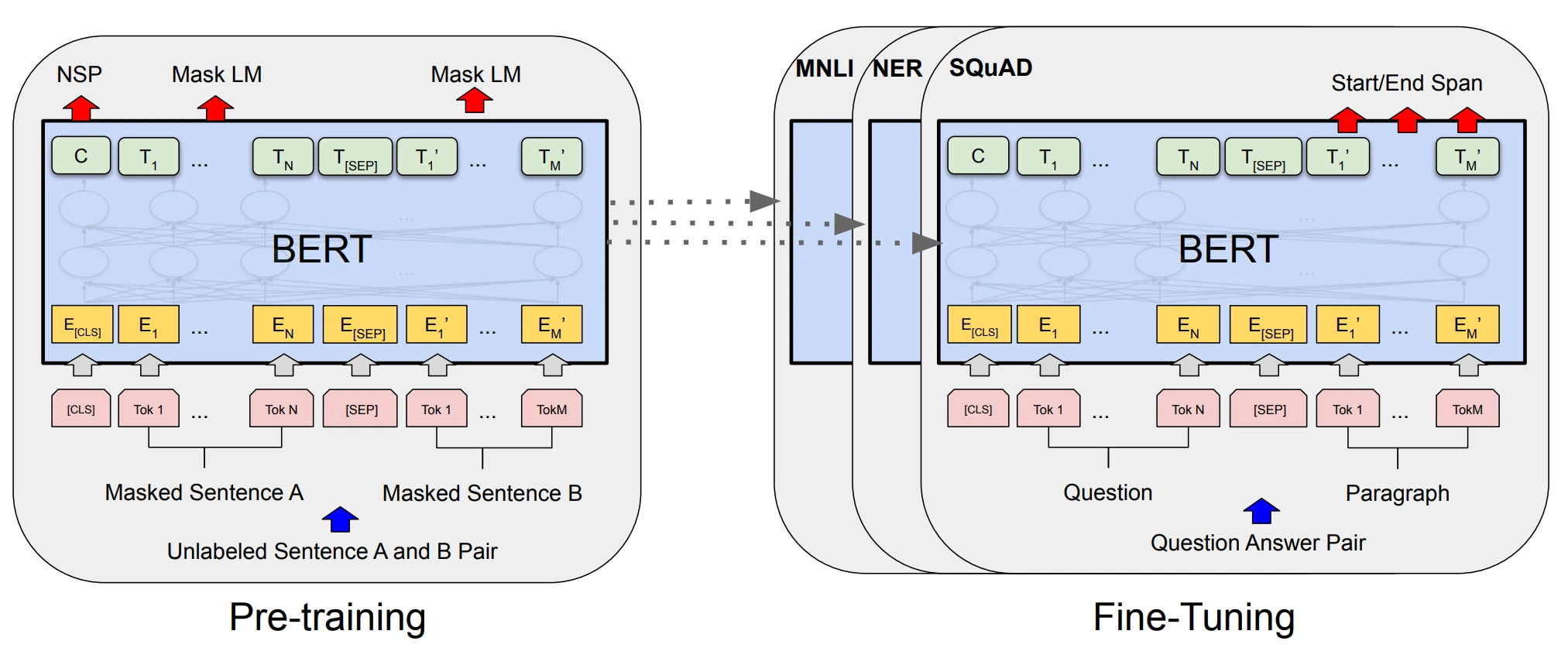 Image taken from the paper
There are a lot of new terms from the above image like CLS, Masked LM, NSP etc that may not make sense at first. But they are quite simple once we understand them. Let us begin
Masked Language Modeling
This is one of the methods of pre-training BERT. We take the input sentence and randomly mask out 15% of the tokens, then using the output of the position we try to predict what could have been the possible text.
In practice, 80% of the times the token is masked, 10% of the times it is replaced with a random token and other 10% of the time it’s left unchanged.
Let’s see this in action:
- Original: “The cat sat on the mat”
- Masked: “The cat [MASK] on the mat”
- BERT sees both “The cat” and “on the mat” to predict “sat”
This bidirectional context is why BERT became so powerful for understanding tasks.
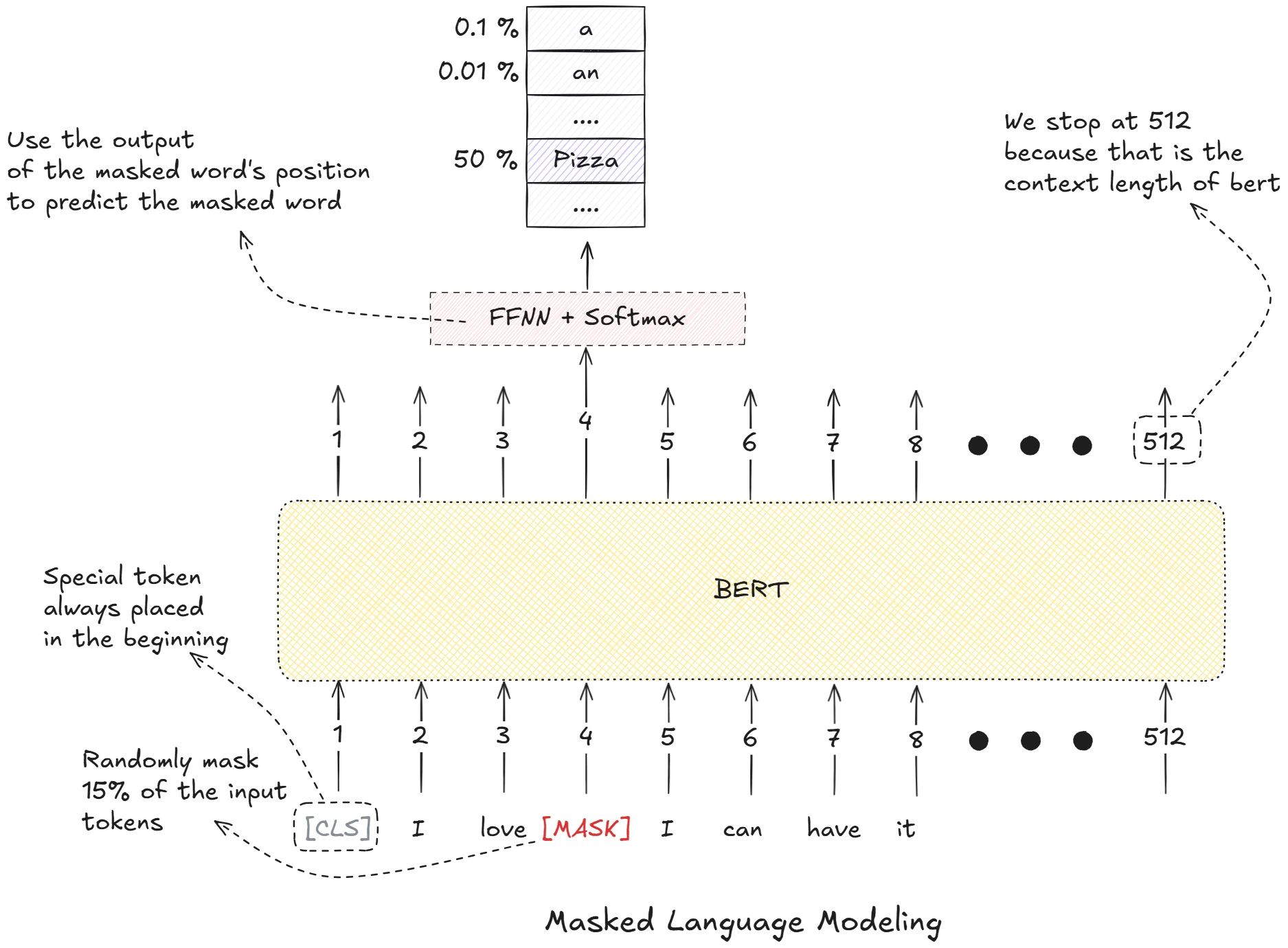
Next Sentence Prediction
Next Sentence Prediction is exactly what it sounds like, but instead of predicting the next sentence. We predict if the given next sentence will come after the first sentence.
The special token CLS learns representation from the both the sentences and the output from it’s position is used to predict whether the sentence comes next or not. In practice, the CLS token is fine tuned for classification, sentiment analysis etc. SEP is a special token that acts as a seperator between both the sentences.
In reality, both NSP and MLM are done simultaneously.
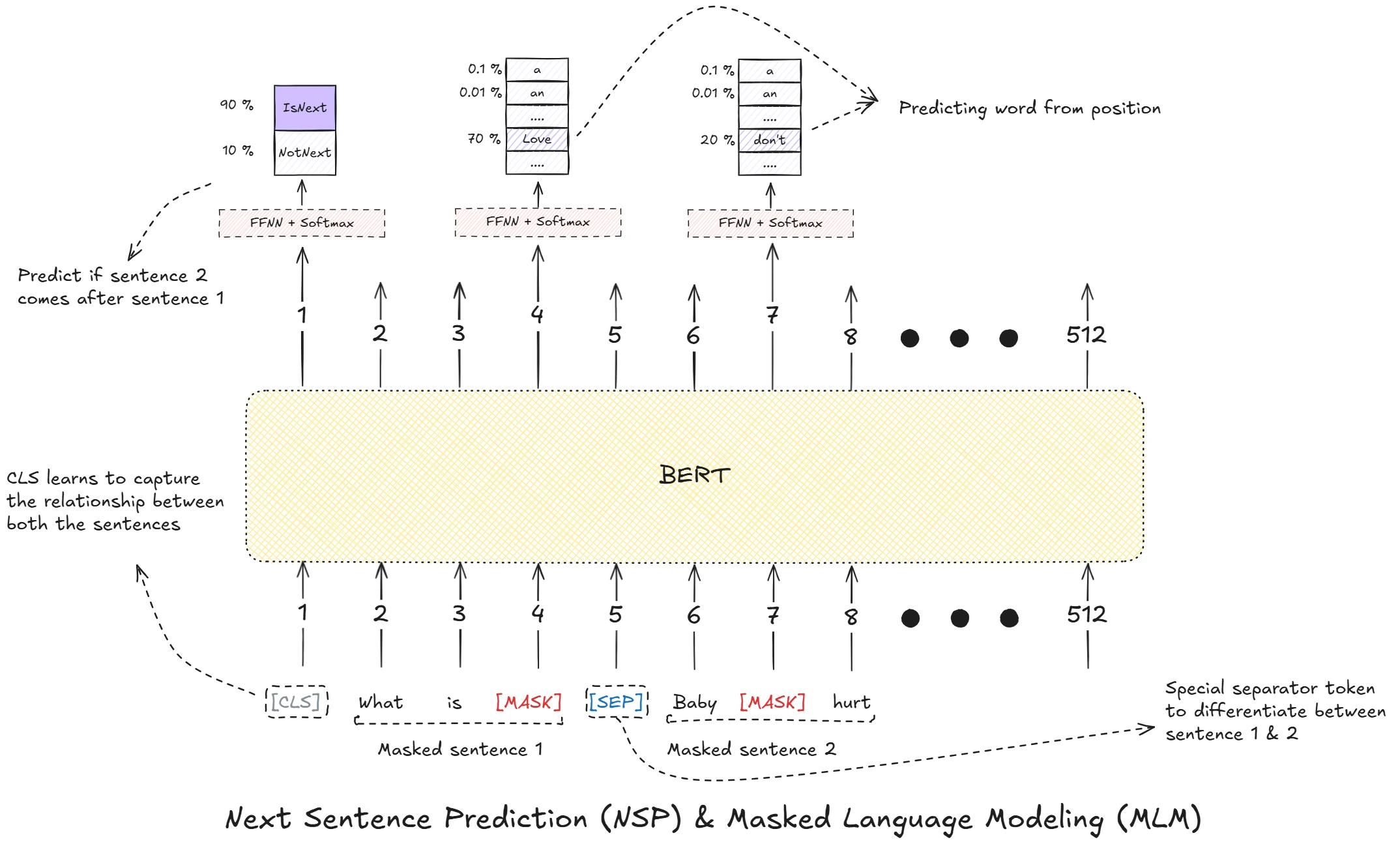
Fine-Tuning
The BERT paper is quite accessible, and has great visuals too. The below image is directly taken from it and shows that to fine tune we just use a small set of training data with labels to fine-tune bert for a specific task.
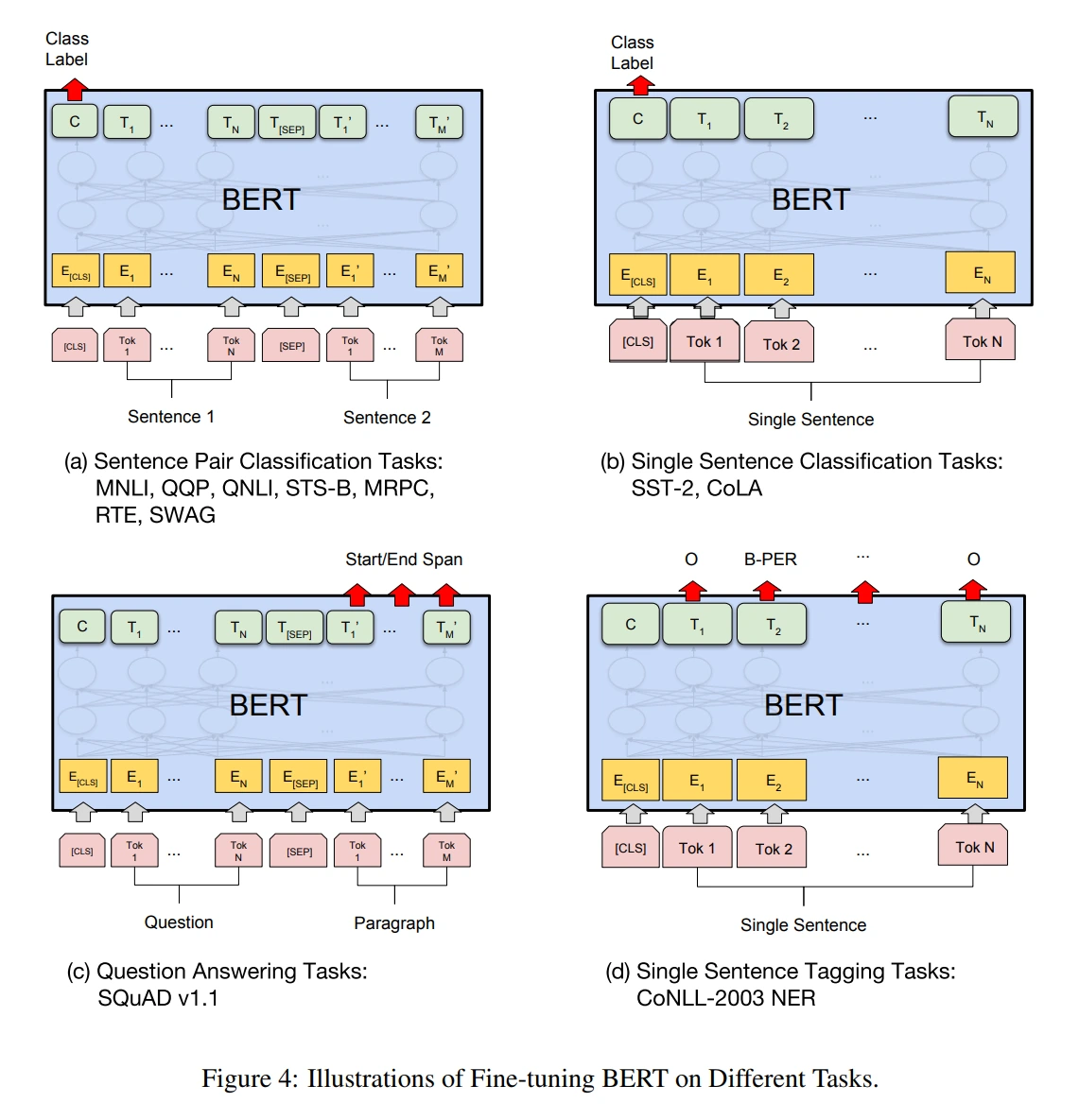
We can use bert to generate embeddings too!! Much like the way we did with ELMo. How? well I leave that upto you to explore.
Why BERT was Revolutionary
Before BERT, each NLP task needed its own specialized architecture. Question answering systems, sentiment classifiers, and named entity recognizers all looked completely different. BERT changed this by providing a universal representation that could be fine-tuned for any task with just a small additional layer.
And that concludes BERT too, now we have talked about the two big architectures of LLMs, moving forward we will mostly be talking about the innovations done in the architecture and the solutions found to increase the scale at which to train them.
2019: Scaling and Efficiency
GPT-2
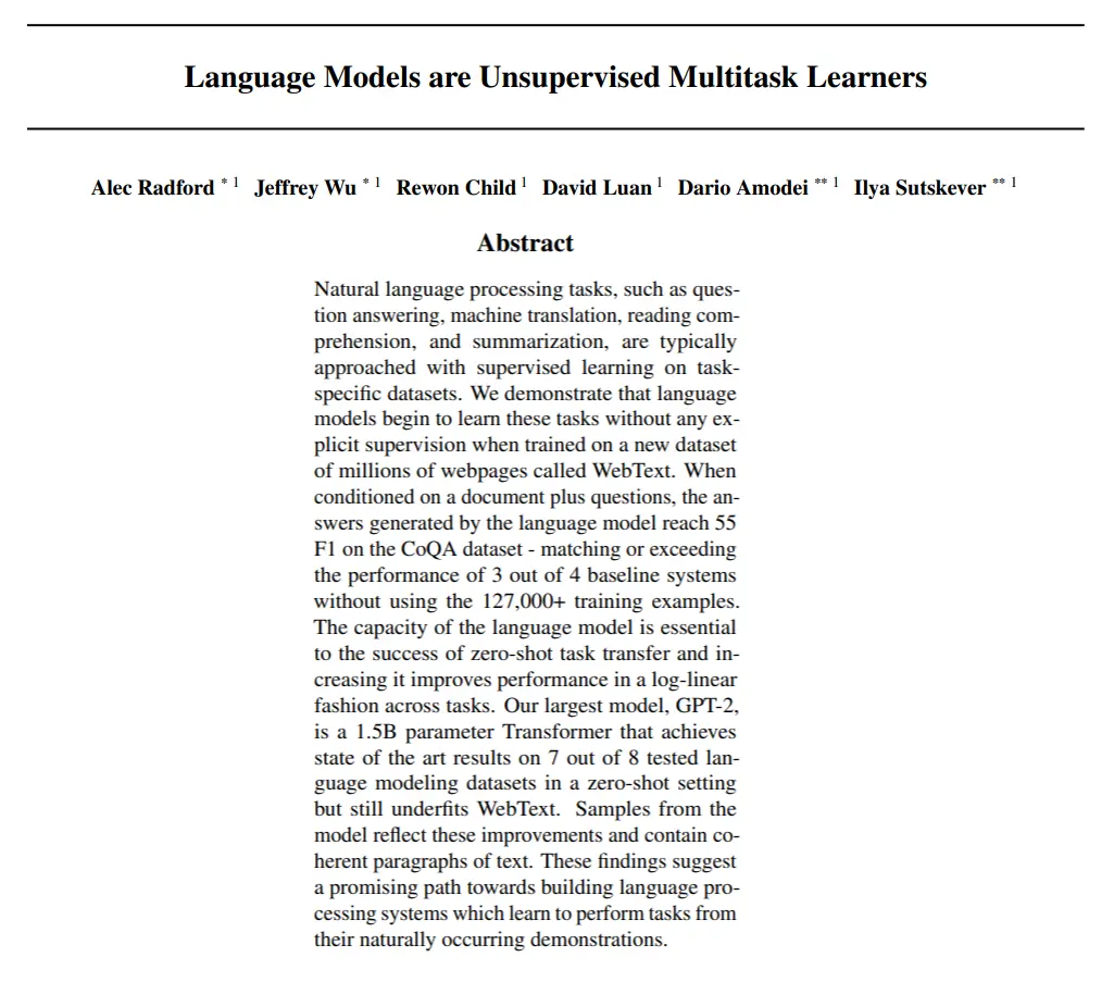
Link to paper: Language Models are Unsupervised Multitask Learners,blog
Quick Summary
This 2019 paper by Radford et al. (OpenAI) introduces GPT-2, a large-scale language model that demonstrates impressive zero-shot learning capabilities across multiple NLP tasks. The key insight of this paper is that language models trained on sufficiently large and diverse datasets naturally acquire the ability to perform various language tasks without explicit supervision.
Key contributions:
- Introduction of WebText - a high-quality web dataset created by scraping outbound links from Reddit with at least 3 karma
- Development of GPT-2, a Transformer-based language model with 1.5 billion parameters
- Demonstration that a single unsupervised language model can perform multiple NLP tasks without task-specific training
- Evidence that model performance scales in a log-linear fashion with model size
The paper shows that GPT-2 achieves state-of-the-art results on 7 out of 8 tested Language Modeling datasets in a zero-shot setting. It also demonstrates promising zero-shot performance on tasks like reading comprehension, summarization, translation, and question answering without any task-specific fine-tuning.
This work represents a significant step toward building more general NLP systems that can learn to perform tasks from naturally occurring demonstrations in text, rather than requiring task-specific datasets and architectures for each application.
This was paper was an improvement over the original GPT, and a huge scaling of it
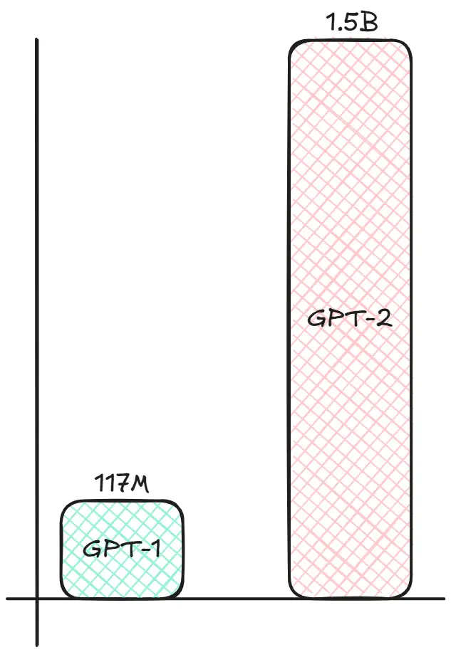
My first question was how did one even get so much data? The authours have underlined that well. So quoting the paper
Common Crawl. Trinh & Le (2018)’s best results were achieved using a small subsample of Common Crawl which included only documents most similar to their target dataset, the Winograd Schema Challenge. While this is a pragmatic approach to improve performance on a specific task, we want to avoid making assumptions about the tasks to be performed ahead of time. Instead, we created a new web scrape which emphasizes document quality. To do this we only scraped web pages which have been curated/filtered by humans. Manually filtering a full web scrape would be exceptionally expensive so as a starting point, we scraped all outbound links from Reddit, a social media platform, which received at least 3 karma. This can be thought of as a heuristic indicator for whether other users found the link interesting, educational, or just funny. The resulting dataset, WebText, contains the text subset of these 45 million links. To extract the text from HTML responses we use a combination of the Dragnet (Peters & Lecocq, 2013) and Newspaper1 content extractors. All results presented in this paper use a preliminary version of WebText which does not include links created after Dec 2017 and which after de-duplication and some heuristic based cleaning contains slightly over 8 million documents for a total of 40 GB of text. We removed all Wikipedia documents from WebText since it is a common data source for other datasets and could complicate analysis due to over…
My second question was how do you run such large models economically?
(Obviously I have skipped how do you “train” such large models, as we will be talking about that in the next section)
And the answer came in the form of …
KV Cache!!!
These two blogs helped me immensely while writing this section, check’em out!!! (they have very nice animations)
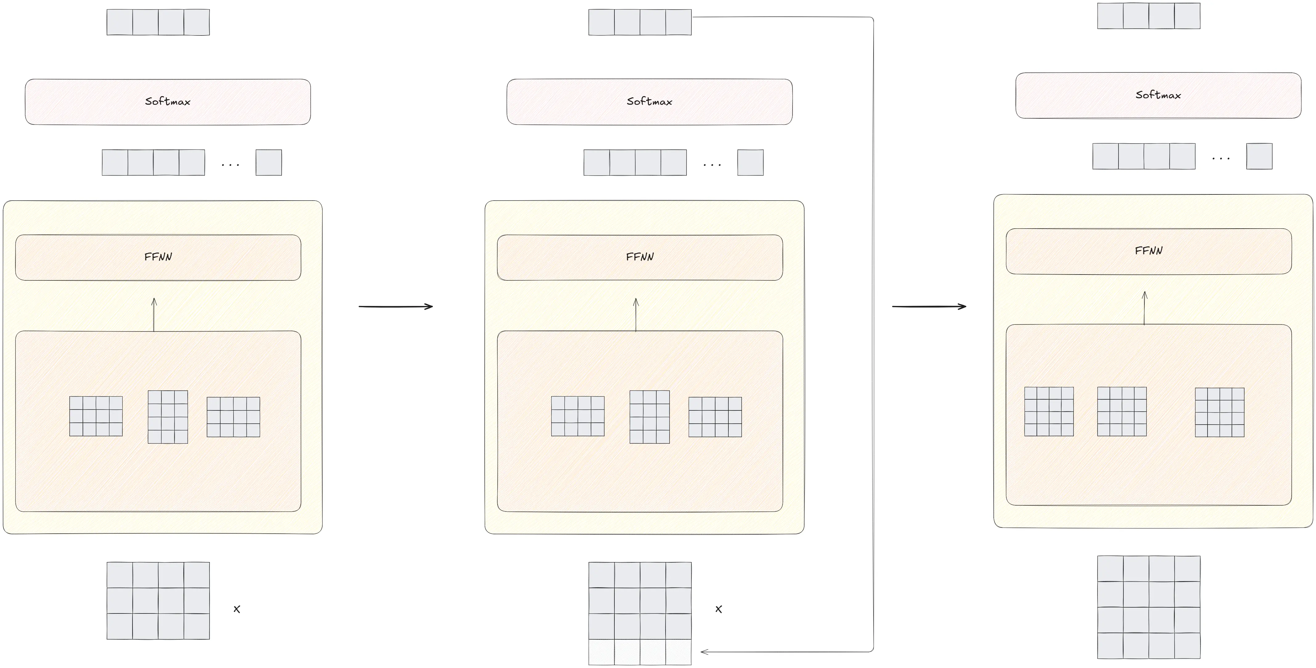
Before we start understanding KV Cache, let us revisit our inference to see what happens.
Let’s say we ask the LLM a question. “Captial of India?” (we already know what happens inside an LLM so I have skipped a lot of the blocks except the essential ones)
Using that, a matrix is formed, for each token id we have embeddings, using which Q,K, and V matrices are made. That gives us our attention values, That is fed to a feed forward network which outputs a vector of logits vocab size, after passing it through softmax let’s say we take the token id with the maximum probability. This gives us a vector output, of token id. (Here I am showing the embeddings)
The embedding of this token is then appended to our original input X, and this operation is repeated till we run into the
Now if we do not cache anything, these values need to be calculated again and again whenever a new token is added as shown above
But we only need to get the attention value for the latest query, we can save the previously calculated queries. (If you are having a hard time thinking why? I will explain it in a while. Hint: Masked Causal attention)
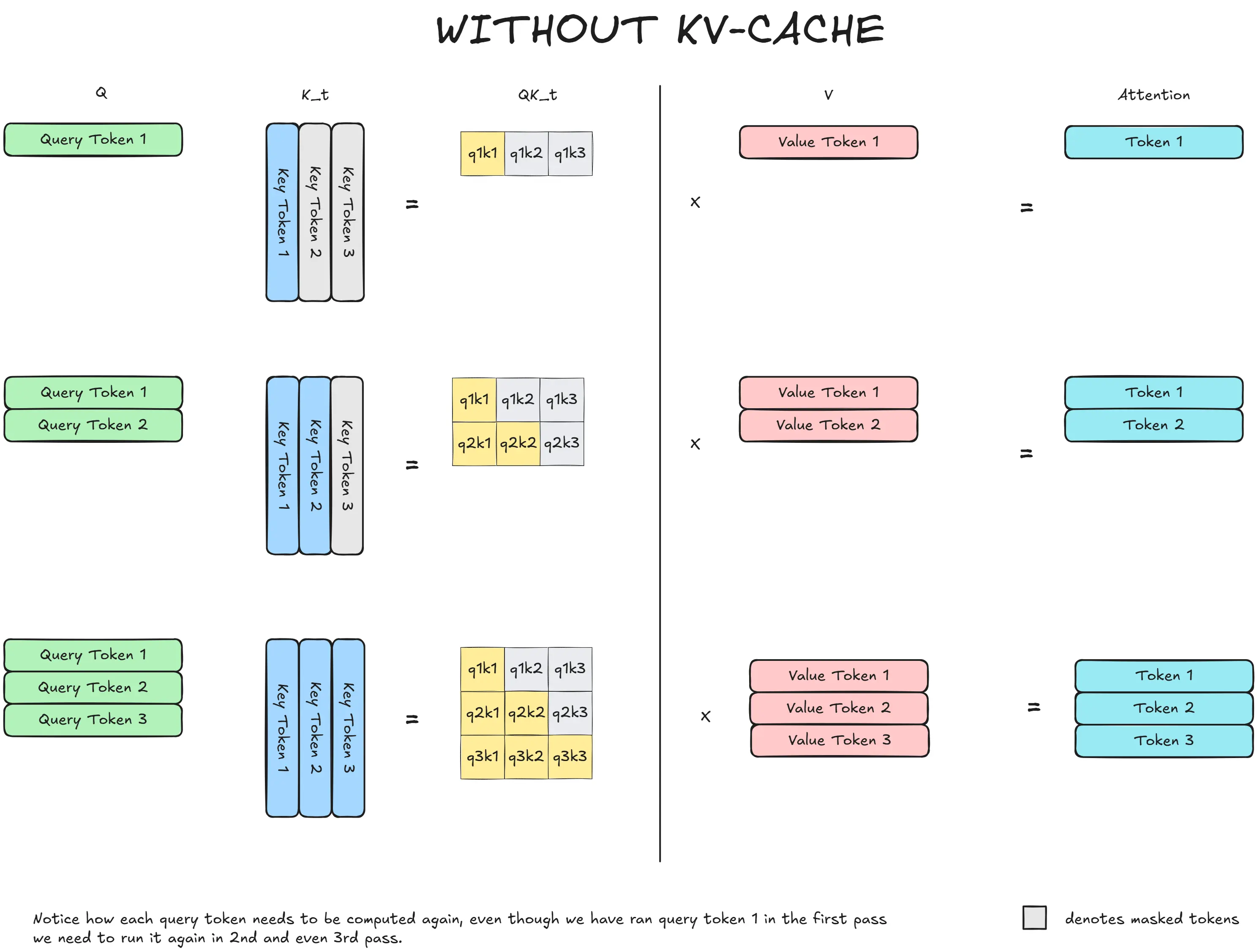
Let’s look closer at the attention calculation itself, If we go vector by vector. We can see that we need to compute $QK^t$ again and again, each time a new token is calculated.
But we do not need to do this for a decoder, as previous tokens never attend to the future tokens. We can just cache the attention of previous tokens and compute the attention score for the latest token!
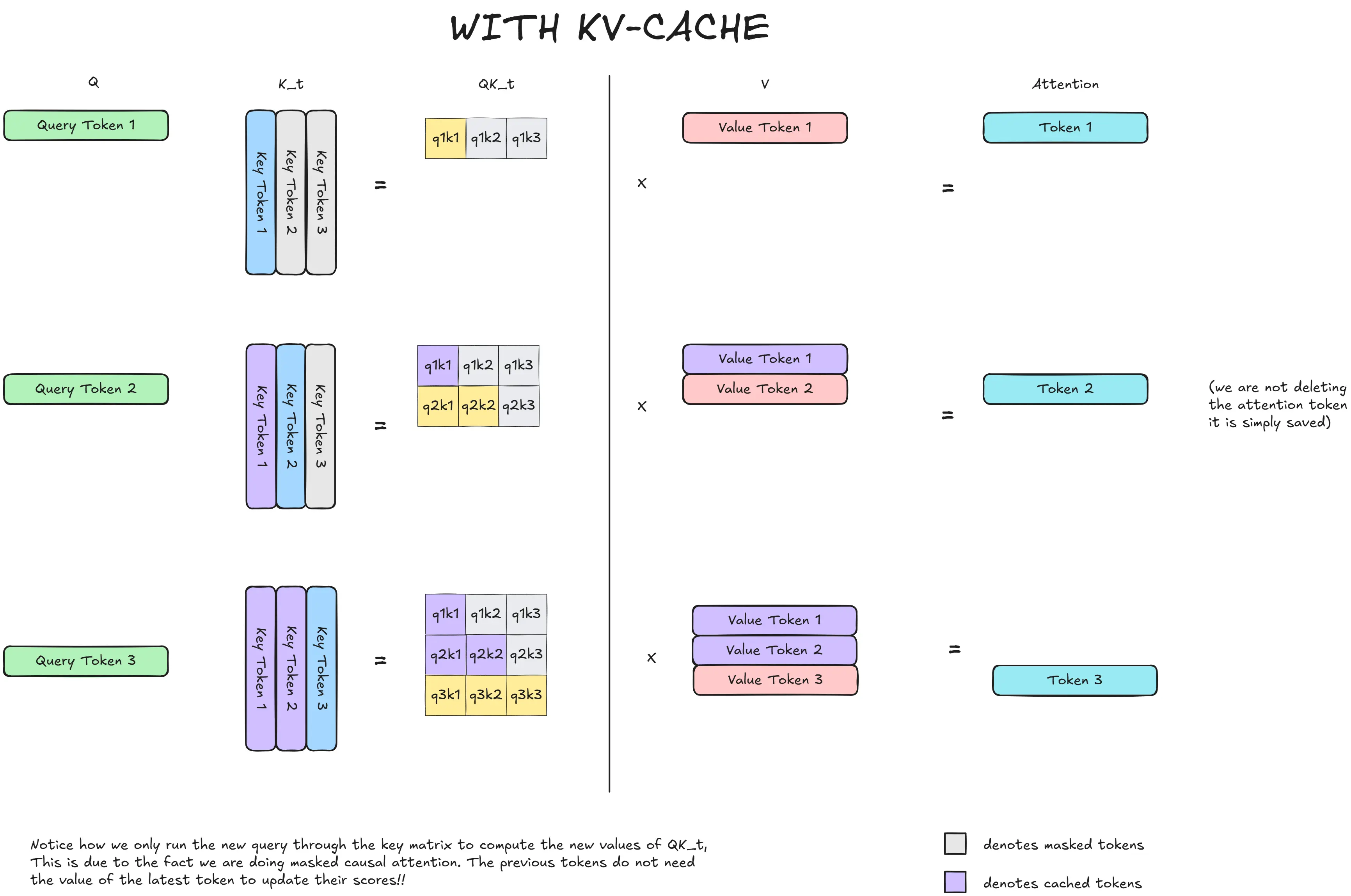
I had two interesting discoveries during this:
- We only cache $K$ and $V$ not $Q$. Because there is no point storing it. To calculate the latest attention score we need the entire $K$ and $V$, but not $Q$. For nth token $Q$, we need the entire of K to calculate $QK^t$. Then we need to multiple the entire $V$ to get the latest attention score. (This is definitely tough to think about, pause take a moment and image it)
- When we append another vector, the shape of $K$ and $V$ also change. But we do not calculate the values of old $Q$ with these because of our masking (We do not need to see the future values), $Q_1$ has no point being multiplied with $K_4$ as that will be masked as infiti anyhoo (We have already talked about this).
The second point also gives us another amazing point, KV caching is not possible in models like BERT (Think why?)
P.S. KV-Cache was not introduced in gpt-2 but became wildly popular after it. I am not able to find the source of the idea. Comment down below if you know about it!!!
That pretty much covers the amazing things that the GPT-2 paper talked about, Let’s move on to see how we can train such big models.
RoBERTa
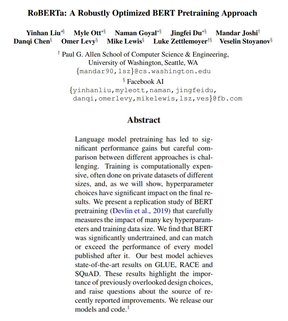
Link to paper: RoBERTa: A Robustly Optimized BERT Pretraining Approach
Quick Summary
This 2019 paper by Liu et al. from Facebook AI presents RoBERTa (Robustly Optimized BERT Pretraining Approach), which demonstrates that BERT was significantly undertrained and can achieve state-of-the-art performance with careful optimization choices.
Key contributions:
-
The paper identifies several critical design decisions that significantly improve BERT’s performance:
- Training the model longer with larger batches over more data
- Removing the Next Sentence Prediction (NSP) objective
- Training on longer sequences
- Dynamically changing the masking pattern applied to training data
-
The researchers collect a larger dataset (including a new CC-NEWS corpus) to better control for training set size effects.
-
Through extensive experimentation, they show that when properly optimized, BERT’s masked Language Modeling objective is competitive with newer approaches like XLNet.
-
RoBERTa achieves state-of-the-art results on GLUE, RACE, and SQuAD benchmarks without multi-task fine-tuning for GLUE or additional data for SQuAD.
The authors emphasize that seemingly mundane training decisions (like batch size, training time, and dataset size) can have as much impact on final performance as architectural innovations. This raises important questions about the source of improvements in recent NLP models and highlights the need for careful replication studies.
The paper is particularly notable for its thorough empirical analysis of training hyperparameters and careful ablation studies showing the contribution of each modification to overall performance.
Problem
The authors found that most of the models released post BERT were challenging to train, hard to compare and they were mostly working as a black box and it was difficult to tell which hyper-parameter were significant. RoBERTa was a replication study on BERT to better understand it. And they unearthed that BERT was significantly under trained.
Solution
- Present a set of important BERT design and training strategies
- Introduction of a novel dataset (CCNEWS)
Dynamic Masking
While training BERT a static masking strategy is employed. I.e the same words are masked throughout training, This can lead to the model memorizing these positions instead of generalizing and learning the relationship between words.
Dynamic masking was a method made to mitigate this issue by varying the masked positions in each epoch. This lead to greater generalization and better performance.
Gradient Accumulation
These two blogs helped me out with this part:
It is well known that mini-batch descent produces good results, but sometimes even the mini batch is large in some cases. Like for CV on a 4k image etc. In those scenarios when we lack memory we use Gradient Accumulation to overcome that issue.
Instead of updating the model in every mini batch, we accumulate the gradient over the course of a few batches then update it.
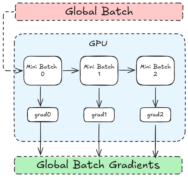
This essentially acts like a bigger batch
A typical training loop looks like this
for inputs, labels in data_loader:
    output = model(input)

    loss = criterion(output,labels)

    loss.backward()
    optimizer.step()
    optimizer.zero_grad()
But when we do gradient accumulation it looks something like this
acc_steps = 3

for idx, (inputs, labels) in enumerate(data_loader):
    output = model(input)

    loss = criterion(output,labels)

    loss.backward()

    # Only do update the weights if it the last mini batch
    if ((idx + 1) % acc_steps == 0) or (idx + 1 == len(data_loader)):
        optimizer.step()
        optimizer.zero_grad()
Large Batch Training
The authors also noted that large batch training can improve training without the need to do complex techniques.
A quote from the paper
Large batch training can improve training efficiency even without large scale parallel hardware through gradient accumulation, whereby gradients from multiple mini-batches are accumulated locally before each optimization step.
Gradient Checkpointing
There really is no reason to mention this here, But this is a popular method to overcome memory limitations too. So I though I will briefly talk about it.
It is rather straightforward, We know when we train a NN, we need to store the gradients for backpropagation. For large models this can get quite big.S So for some layers instead of storing it, we re-compute it during backprop.
(Obviously much more goes into training the large scale LLMs we use nowdays, we will talk about them as we move forward)
DistilBERT and Model Compression
Link to paper: DistilBERT, a distilled version of BERT: smaller,faster, cheaper and lighter
Quick Summary
This 2020 paper by Sanh et al. from Hugging Face introduces DistilBERT, a smaller, faster version of BERT created through knowledge distillation. The authors address the growing concern that state-of-the-art NLP models are becoming increasingly large and computationally expensive, limiting their practical deployment, especially on edge devices.
Key contributions:
-
They create a distilled version of BERT that retains 97% of its language understanding capabilities while being 40% smaller and 60% faster at inference time.
-
DistilBERT is built using knowledge distillation during the pre-training phase (rather than task-specific distillation), using a triple loss function that combines:
- The standard masked Language Modeling loss
- A distillation loss using the teacher’s soft target probabilities
- A cosine embedding loss to align the directions of the student and teacher hidden states
-
The student model (DistilBERT) uses the same architecture as BERT but with half the number of layers, and is initialized by taking every other layer from the teacher model.
-
The authors demonstrate that DistilBERT performs well across various NLP tasks:
- On GLUE benchmark tasks, it retains 97% of BERT-base’s performance
- On IMDb sentiment classification, it achieves 92.82% accuracy (vs. 93.46% for BERT-base)
- On SQuAD question answering, it reaches 85.8 F1 (vs. 88.5 for BERT-base)
-
They also show that DistilBERT can run effectively on mobile devices, with a model size of 207 MB and 71% faster inference time than BERT on an iPhone 7 Plus.
This work demonstrates that through careful distillation, smaller and more efficient models can be created without significant loss in performance, making state-of-the-art NLP more accessible for resource-constrained applications.

The following sources helped me immensely while writing this section.
- Survey paper on Knowledge Distillation
- HuggingFace Blog on Knowledge distillation
- Blog by the creators of distillbert
What is Knowledge Distillation
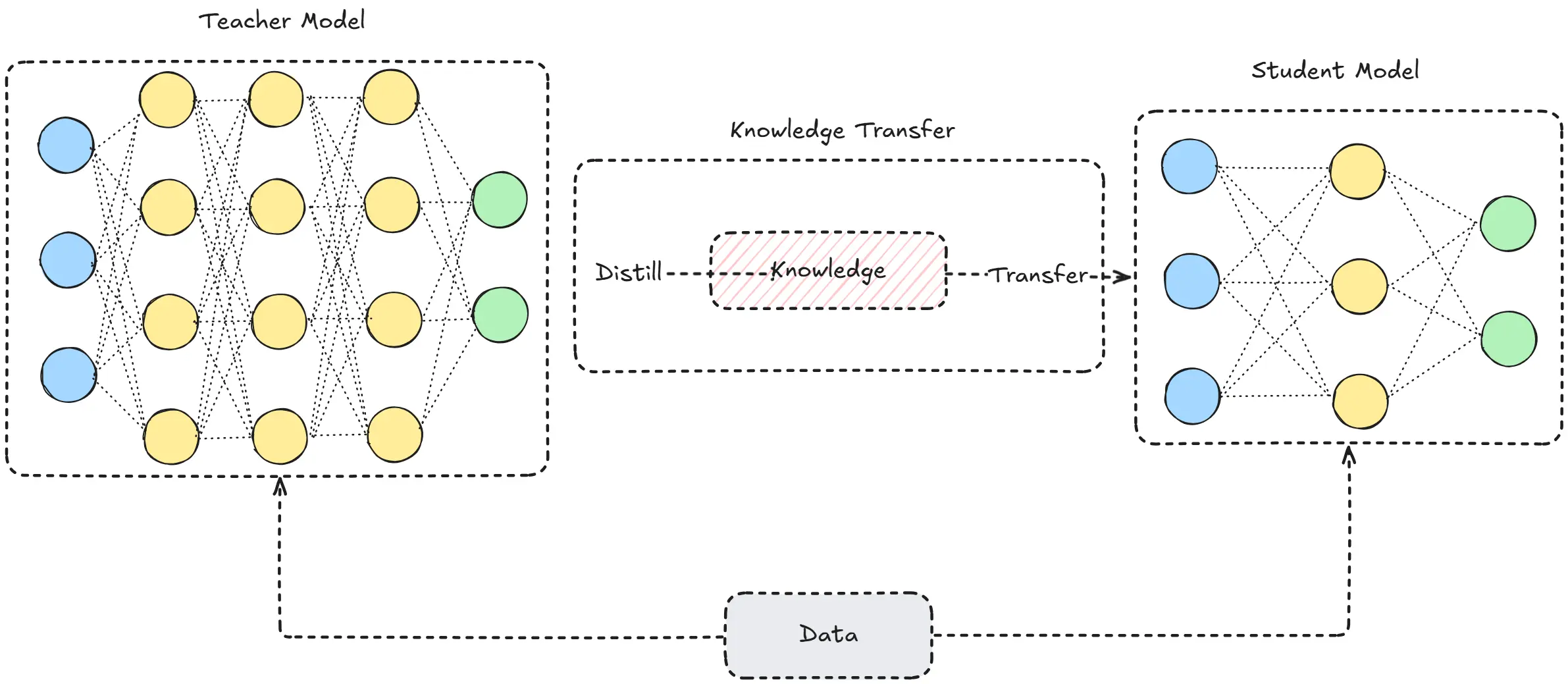
The idea is quite simple we have a big heavy model trained for long period of time on a lot of data, and we want a smaller model to learn from the bigger model.
There are many reasons we may wish to do this, they are cheaper and faster to inference. They can on edge devices like mobiles, watches, drones etc. And most of the times they retain 90+ performance of the original model while being significally smaller.
Types of Knowledge Distillation
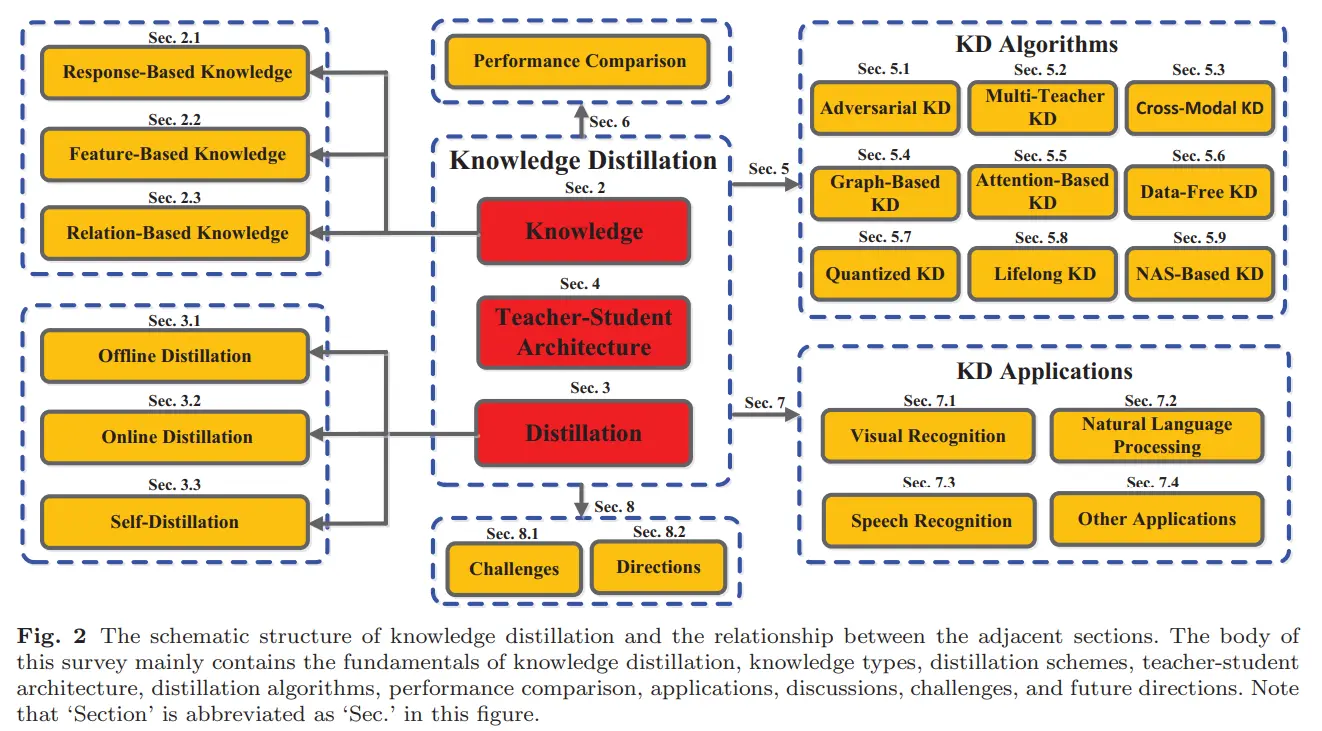 Image taken from paper
There are definitely many kinds of distillation methods available to us (the above image makes it quite obvious). We will not be able to talk about all of them, So I will touch on the most popular one’s and ask you to explore the one’s you find interesting.
Response Based
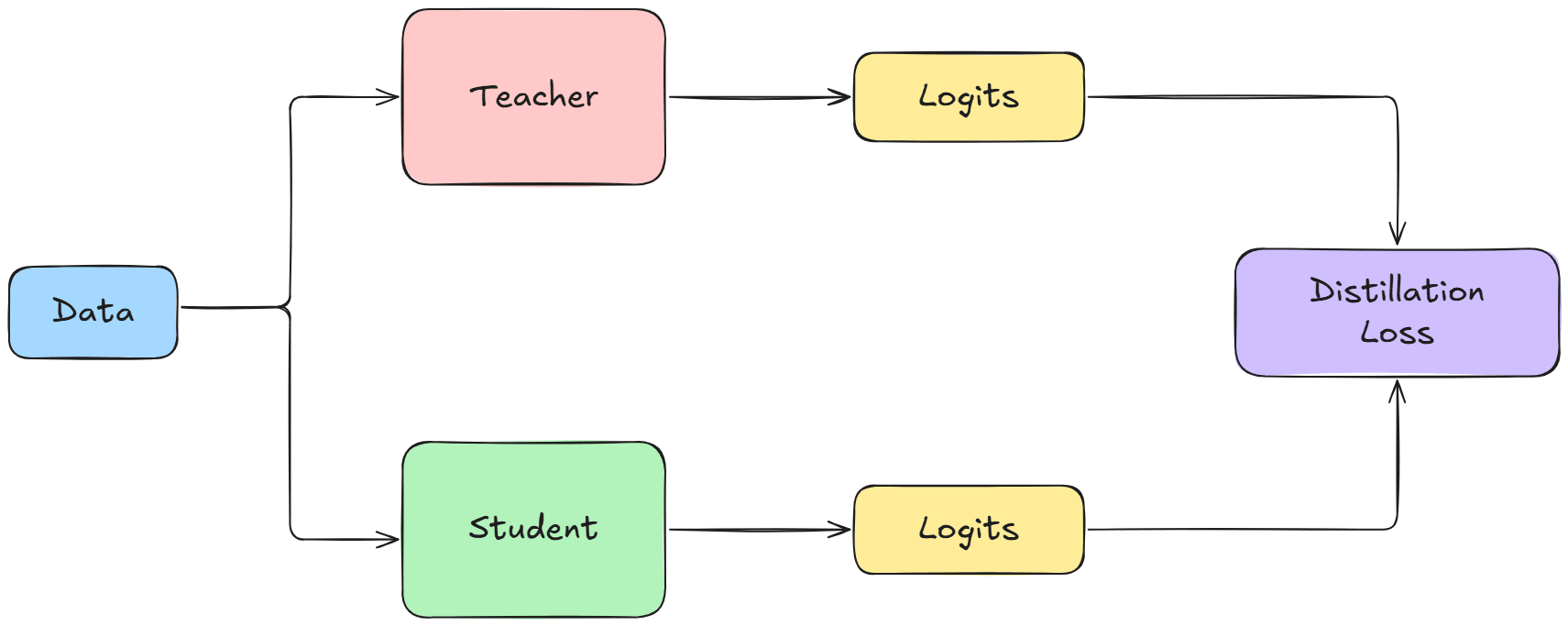
In this method, we take a sample of training data. Run it by both our models. And then make the smaller model learn the soft labels of the bigger model.
We are essentially trying to make the smaller model predict like the bigger model.
Now one may question what are soft labels, Lets see it with an example
[0,1,0,0] -> hard labels
[0.1,0.3,0.5,0.1] -> soft labels
A model outputs an array of probabilities, out of which many are near zero probabilities. These near zero probabilities still hold a lot of knowledge
For instance an apple can be confused for a red ball, but it should not be confused for the moon.
This is known as dark knowledge. We are essentially trying to make our smaller model learn this dark knowledge.
Hinton et al introduced an idea of temperature to control the importance of these soft labels. As T tends to inifity all latels have the same value
\[p_i = \frac{\exp(z_i/T)}{\sum_j \exp(z_j/T)}\]Where:
- $p_i$ is the probability of class $i$
- $z_i$ is the logit for class $i$
- $T$ is the temperature parameter
Temperature $T$ controls how “soft” the probability distribution becomes. When $T = 1$, we get the normal softmax. As $T$ increases, the distribution becomes more uniform (softer), revealing the relative similarities between classes that the teacher model has learned. When $T → ∞$, all probabilities approach equal values. During distillation, we use $T > 1$ to extract this “dark knowledge” from near-zero probabilities.
Feature Based
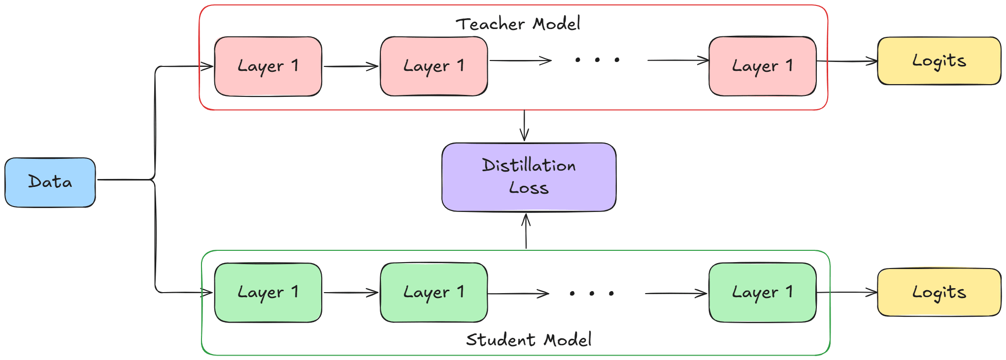
In this, we hope to replicate the weights of the bigger model in our smaller model. Instead of matching final outputs, we match intermediate representations (feature maps) from corresponding layers of teacher and student models. The student learns to produce similar internal representations as the teacher, capturing how the teacher processes information at different depths. Transformation functions $\Phi_t$ and $\Phi_s$ may be needed when teacher and student have different dimensions.
\[L_{FeaD}(f_t(x), f_s(x)) = L_F(\Phi_t(f_t(x)), \Phi_s(f_s(x)))\]where:
- $L_{FeaD}$ is the feature distillation loss
- $f_t(x)$ and $f_s(x)$ are the teacher and student feature representations
- $\Phi_t$ and $\Phi_s$ are transformation functions for the teacher and student features
- $L_F$ is the loss function applied to the transformed features
Relation Based
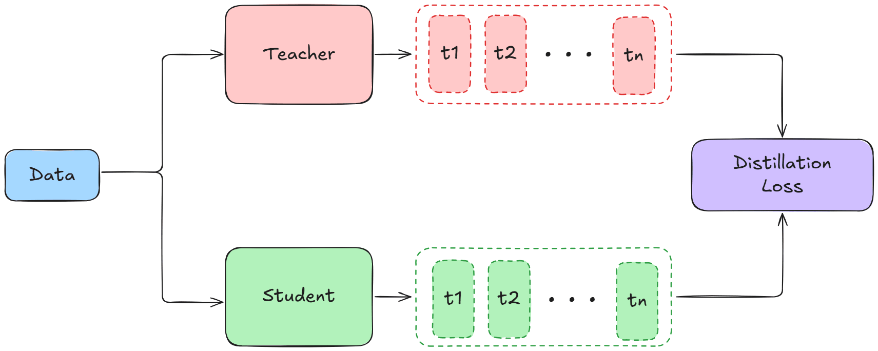
Take a pair of feature maps from both the models, and minimize the loss between their relationship.
NOTE: Even though feature maps is used both in featured based and realtion based KD, they are quite different. For example in Feature based we are trying to map the exact features to be in the same distribution. But in realtion based, the indiividual values do not matter, the realtion between them does. For example in feature based if Ft(Xt) = 5 then we want Fs(X) = 5 as well. But in Relation Ft(x1,x2) = 5 then Fs(x3,x4) = 5 where the feature maps x by themselves can be quite different
As mentioned earlier, there are a lot of methods available for KD. If you are further intersted, checkout the survey!
How was diltillbert trained
Distillbert was trained using the response based distillation method. KLD is used as the distillation Loss.
import torch
import torch.nn as nn
import torch.nn.functional as F
from torch.optim import Optimizer

KD_loss = nn.KLDivLoss(reduction='batchmean')

def kd_step(teacher: nn.Module,
            student: nn.Module,
            temperature: float,
            inputs: torch.tensor,
            optimizer: Optimizer):
    teacher.eval() # Notice teacher model is in eval mode
    student.train()

    with torch.no_grad():
        logits_t = teacher(inputs=inputs) # Do not store the gradients of teacher
    logits_s = student(inputs=inputs)

    loss = KD_loss(input=F.log_softmax(logits_s/temperature, dim=-1),
                   target=F.softmax(logits_t/temperature, dim=-1)) # KLD loss on teacher output with student output.
                   # Notice how the student output is a log softmax, because we are training it

    loss.backward()
    optimizer.step()
    optimizer.zero_grad()
Code modified from gist
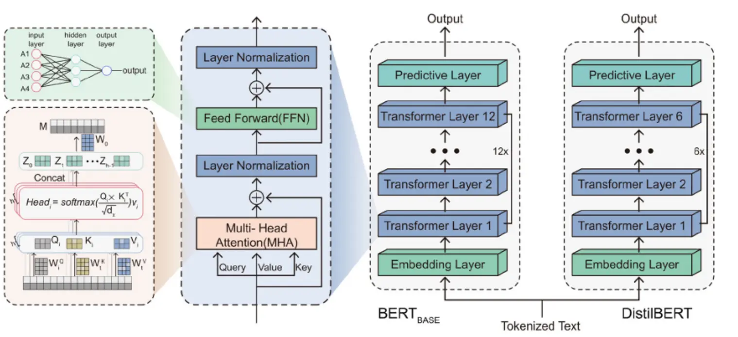
The architecture of distillbert is very similar to BERT, they have reduced the number of layers. Significantly decreasing the amount of parameters (From 110M to 66M), While maintaing 95% performance of BERT. The authors additionally removed the token-type embeddings and the pooler (as there is no Next sentence predition here)
It is interesting to talk about the initialization and training as well. As noted by the author they initialized distillbert by taking the weights of every other layer (as they had common hidden size namely 768). They also trained the model on very large batches, using gradient accumulation, with dynamic masking and NSP removed.
Now let’s talk about the loss used to train DistillBert. They used a triple loss which is a combination of MLM Loss, Distillation Loss & Similarity Loss.
These Beautiful images were taken from this blog
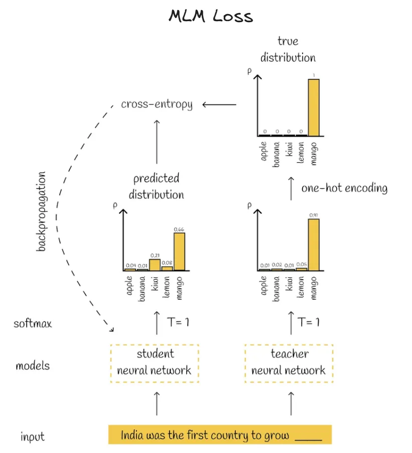
Masked Language Modeling Loss is pretty straight forward and we have already talked about it in our BERT section. In this we do cross entropy over predicted distribution and true distribution.
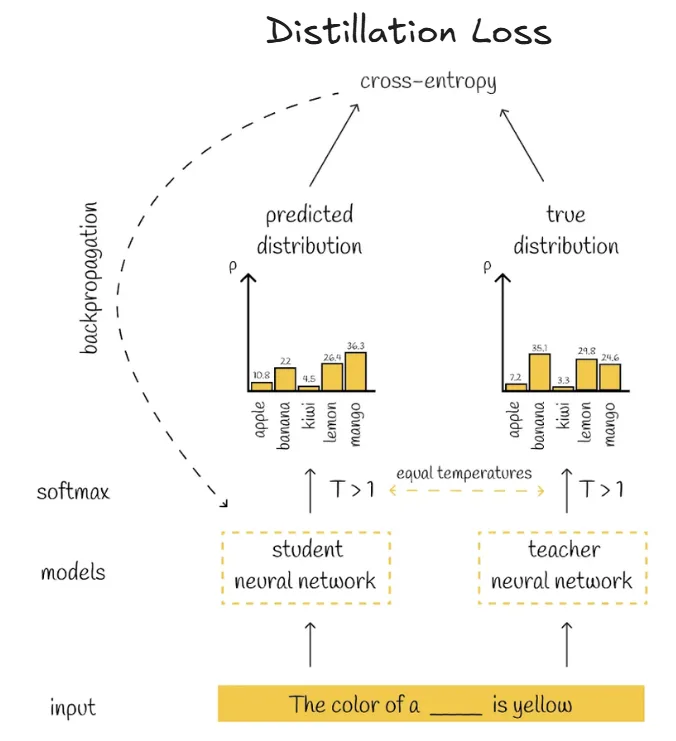
Distillation loss is an idea that is new here, it is a response based loss, In which we compare the KLD between the Teacher’s output distribution and the Student’s output distribution.
Here KLD and Cross-Entropy has been used interchangably, but that is usually not the case.
KLD and cross-entropy can be used interchangeably only when the one distribution is fixed (Here the teacher distribution). Here’s why:
\[\text{KLD}(p_{teacher} || p_{student}) = \sum_i p_{teacher}(i) \log \frac{p_{teacher}(i)}{p_{student}(i)}\] \[= \sum_i p_{teacher}(i) \log p_{teacher}(i) - \sum_i p_{teacher}(i) \log p_{student}(i)\]Since the teacher’s distribution is fixed during training, the first term $\sum_i p_{teacher}(i) \log p_{teacher}(i)$ is constant and can be ignored for optimization purposes. The remaining term $-\sum_i p_{teacher}(i) \log p_{student}(i)$ is exactly the cross-entropy loss. Therefore, minimizing KLD is equivalent to minimizing cross-entropy in this context.
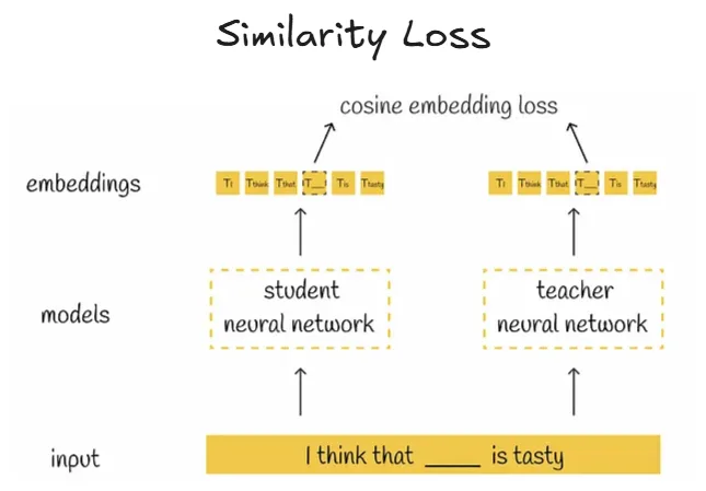
Cosine embedding loss is straight forward as well, here we just take the cosine distance between the embedding vector.
Remember the embedding matrix is also a learned parameter!
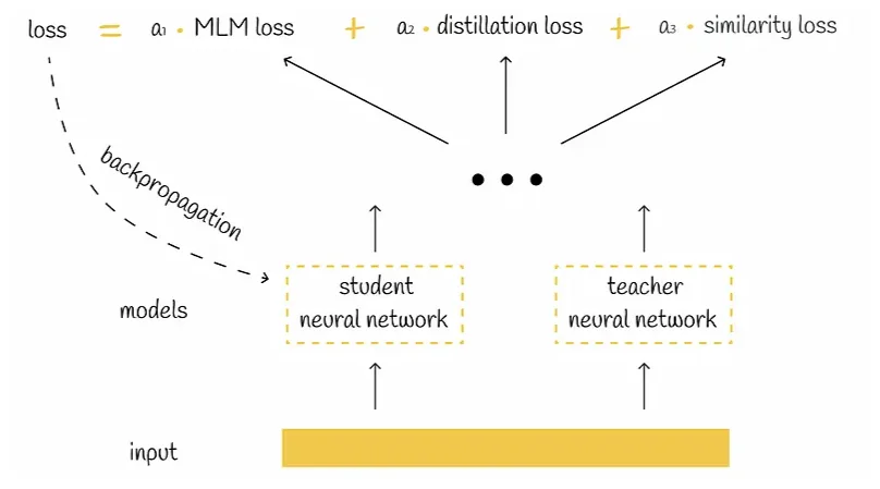
In the end, we put all of it together and train DistillBERT!!!
If you would like to distill a model, this is a good tutorial by PyTorch. Furthermore this was a nice paper on distillation scalling laws, consider checking it out!
BART
Link to paper: BART: Denoising Sequence-to-Sequence Pre-training for Natural Language Generation, Translation, and Comprehension
Quick Summary
The paper introduces BART (Bidirectional and Auto-Regressive Transformers), a denoising autoencoder for pretraining sequence-to-sequence models. BART works in two stages:
- It first corrupts text with various noising functions (like token masking, deletion, text infilling, sentence shuffling)
- Then it learns to reconstruct the original text
BART combines the bidirectional encoding approach of BERT with the autoregressive generation capabilities of GPT. This architecture makes it particularly effective for both text generation and comprehension tasks. The authors evaluate various noising approaches and find that randomly shuffling sentences combined with a novel text infilling scheme (replacing spans with mask tokens) works best.
In experiments, BART achieves strong performance across multiple NLP tasks:
- Matching RoBERTa on classification tasks like GLUE and SQuAD
- Achieving new state-of-the-art results on summarization tasks (with up to 6 ROUGE point improvements)
- Showing effectiveness for dialogue, question answering, and even machine translation
The paper presents a thorough ablation study comparing BART to other pretraining approaches and demonstrates its versatility as a general-purpose language model.
BART is not as complex as the ideas we have discussed so far, reading the summary above should be enough.
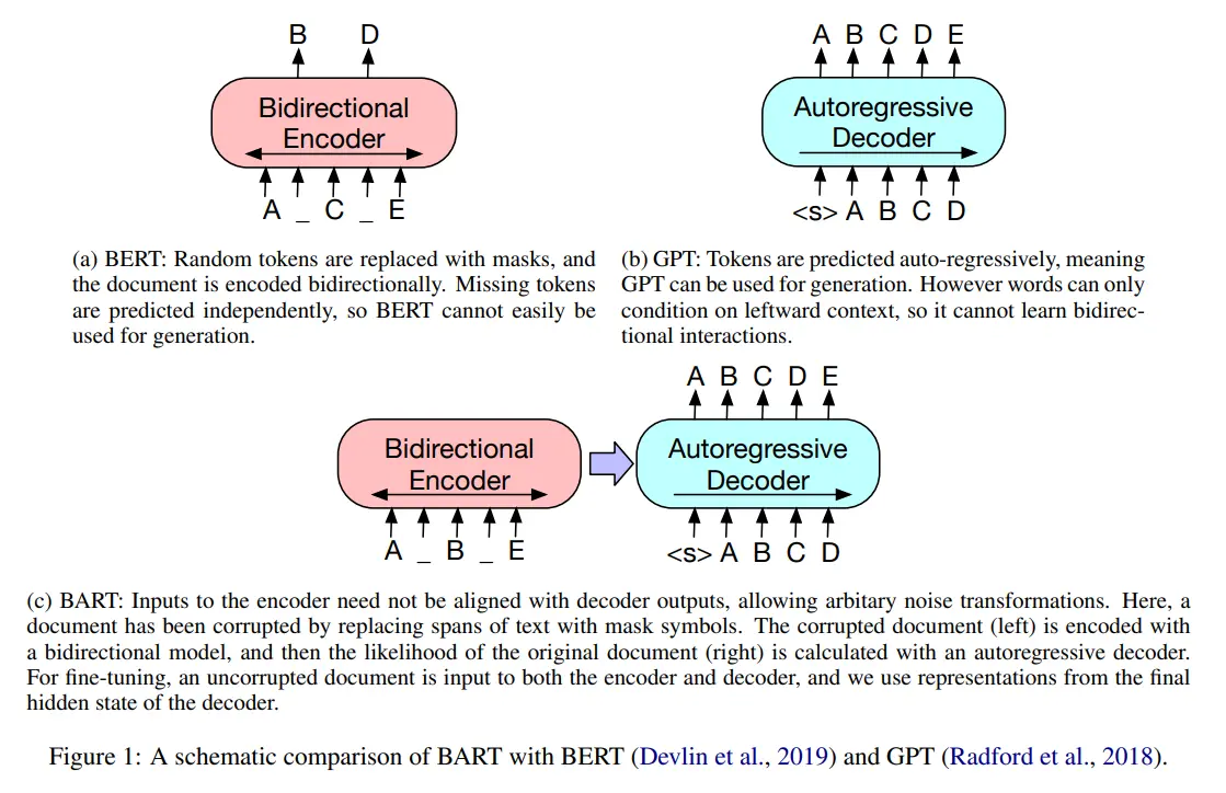
In simple terms BART is just BERT + GPT. The novel idea it introduced was in it’s training. Where corrupted data was given as the input and using reconstruction loss (Cross entropy over predicted and original data distribution), the outputs were predicted.
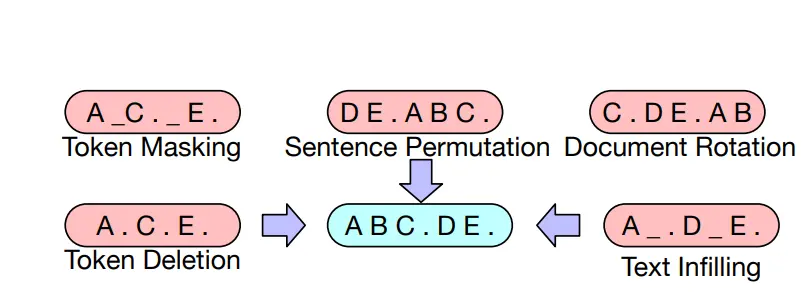
Most of the noise and corruption is self explanatory from the above image, except text infilling. So let us talk about that for a moment.
In it we take a text (Pizza is the most delicious dish in the world) and we sample a span, whose length is drawn from a Poisson distribution ($\lambda=3$). These spans (Pizza is/delicious/in the world) are then masked ([MASK] the most [MASK] dish [MASK]).
In the current age, The BART architecture never gained popularity. I believe partly due to it’s complexity. There is nothing else left to discuss so I’ll be skipping the fine-tuning method. If you wish to know more about it, consider going through the paper.
Transformer-XL
Link to paper: Transformer-XL: Attentive Language Models Beyond a Fixed-Length Context
Quick Summary
This paper introduces Transformer-XL, a novel neural architecture that addresses a key limitation of standard Transformers in language modeling: their inability to capture dependencies beyond a fixed context length.
Key Problems Solved
Context Fragmentation: Traditional Transformers process text in fixed-length segments without information flow between segments, leading to inefficient optimization and poor prediction of tokens at segment boundaries.
Limited Dependency Length: Vanilla Transformers can only model dependencies within their fixed context window, typically a few hundred tokens.
Main Innovations
- Segment-Level Recurrence Mechanism
- Reuses hidden states from previous segments as extended context for the current segment
- Enables modeling of much longer dependencies (80% longer than RNNs, 450% longer than vanilla Transformers)
- Creates a recurrent connection between segments while maintaining the parallelization benefits of self-attention
- Relative Positional Encoding
- Replaces absolute positional encodings with relative ones to enable state reuse
- Decomposes attention into four intuitive terms: content-based addressing, content-dependent positional bias, global content bias, and global positional bias
- Allows models trained on shorter sequences to generalize to longer ones during evaluation
Results
Transformer-XL achieved state-of-the-art results across multiple datasets:
- WikiText-103: 18.3 perplexity (previous best: 20.5)
- enwiki8: 0.99 bits per character (first to break 1.0)
- One Billion Word: 21.8 perplexity
- Up to 1,874x faster evaluation speed compared to vanilla Transformers
Technical Contributions
The architecture maintains gradient flow within segments while allowing information to propagate across segments through cached hidden states. The relative positional encoding scheme ensures temporal coherence when reusing states and generalizes well to longer contexts than seen during training.
Impact
Transformer-XL demonstrated the ability to generate coherent text spanning thousands of tokens and established new benchmarks for long-range dependency modeling. The techniques introduced became influential for subsequent developments in large language models, particularly for handling longer contexts efficiently.
The paper represents a significant step forward in extending the effective context length of Transformer-based models while maintaining computational efficiency.
Problem The big problem with vanilla transformers was their fixed context length. During training and inference, they could only pay attention to a limited chunk of text at a time, like reading a book through a keyhole. Any information outside that small window was completely invisible.
This method of splitting text into rigid segments also caused context fragmentation. Imagine a sentence being cut in half between two segments. The model would struggle to understand the beginning of the second segment because it couldn’t see the end of the first one, leading to poor performance and inefficient training.
Solution
- A method to pass information through the segments
- Novel Positional Encoding Scheme
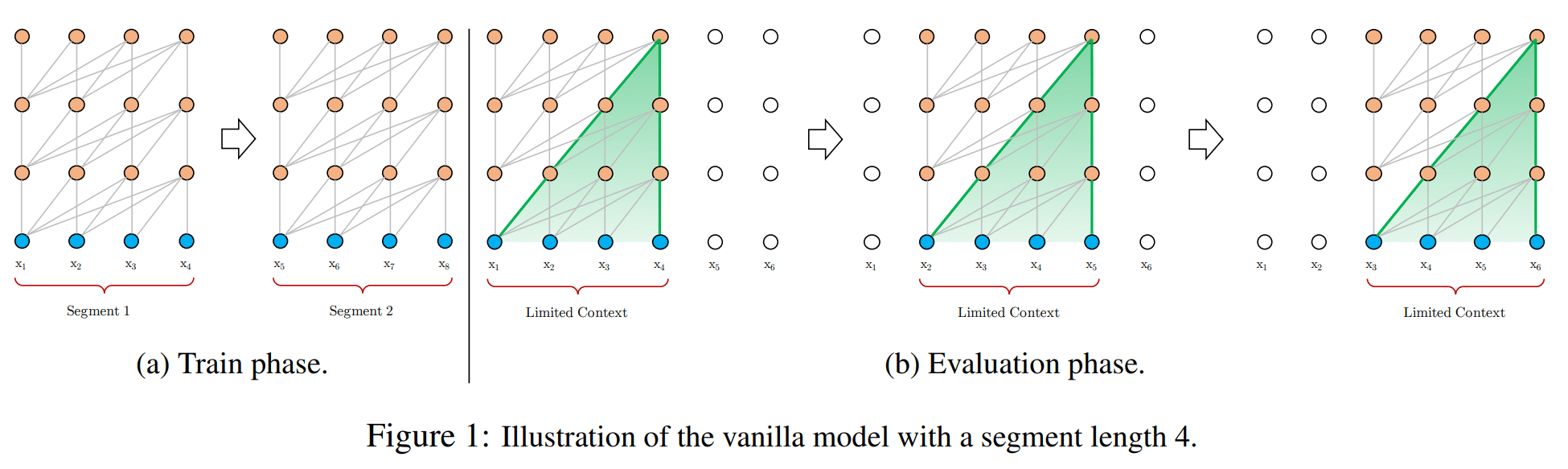
The above image is of a traditional model during it’s train and evaluation phase. Notice the segments, you will see that Segment 2 [$X_5$ to $X_8$] have no information passed from Segment 1 [$X_1$ to $X_4$]. This leads to two problems, first being we can only use our model withing a limited context window, Outside which we won’t be able to run it. The other being of data fragmentation, I.E text data is highly connected and breaking it into segments can break the flow of information (Something present in the first segment which is relevant to the third segment won’t be present in it!)
To solve this problem, the authors introduced two ideas
Segment-level Recurrence
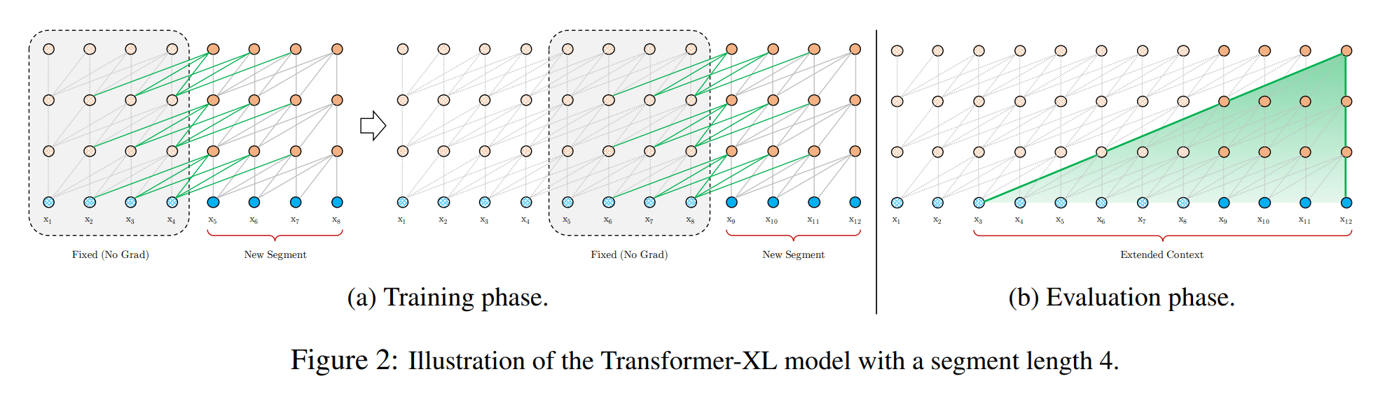
In this during the train phase, after a segment is processed, its calculated hidden states are cached and reused as an extended context for the next segment. When the model processes the new segment, it can attend to both its own tokens and the tokens from the previous segment’s cache.
Crucially, the gradients only flow through the current segment. The cached states are “frozen,” acting as a read-only memory. This allows the model to learn from past information without the massive computational cost of backpropagating through the entire sequence, similar in spirit to truncated backpropagation in RNNs.
Relative Positional Encodings
There is still one minor problem that needs to be addressed. Back then, fixed positional encoding used to be used in models (Read this if you are new to this idea).
It assigns a unique embedding to each position (e.g., position 1, position 2, etc.). This breaks when we introduce recurrence.
- Segment 1 has tokens at positions
1, 2, 3, 4 - Segment 2 also has tokens at positions
1, 2, 3, 4
When we process Segment 2, the model sees the token at absolute position 5 (the first token of Segment 2) and the token at absolute position 1 (the first token of Segment 1). But both are labeled with the same positional encoding for “position 1”. The model has no way to tell them apart, leading to what the paper calls temporal confusion.
And the authors solve it using Relative Positional Encoding. Ok, this part get’s kind of tough, so bear with me as I walk you through step by step
Step 1: The Math of a Standard Transformer
In a standard Transformer, the input for a token at a specific position i is the sum of its word embedding and its positional embedding:
Here, $E_i$ is the word embedding (the token’s meaning), and $U_i$ is the absolute positional embedding (the token’s fixed address in the sequence).
The Query and Key vectors are linear transformations of this input:
\(Q_i = (E_i + U_i)W_q\) \(K_j = (E_j + U_j)W_k\)
The attention score is the dot product of a specific Query vector $Q_i$ with a specific Key vector $K_j$. If we expand this dot product, we reveal four distinct components that the model uses to calculate attention:
\[A_{i,j}^{\text{abs}} = ( (E_i + U_i)W_q )^\top ( (E_j + U_j)W_k )\] \[A_{i,j}^{\text{abs}} = \underbrace{E_i^\top W_q^\top W_k E_j}_{\text{(a) content-content}} + \underbrace{E_i^\top W_q^\top W_k U_j}_{\text{(b) content-position}} + \underbrace{U_i^\top W_q^\top W_k E_j}_{\text{(c) position-content}} + \underbrace{U_i^\top W_q^\top W_k U_j}_{\text{(d) position-position}}\]The problem lies in terms (b), (c), and (d), which all rely on the absolute position vectors $U_i$ and $U_j$. This rigid system breaks when we use recurrence, as the model can’t distinguish between position 5 in segment one and position 5 in segment two.
Step 2: Rebuilding the Attention Score for Transformer-XL
To solve this, Transformer-XL re-engineers the attention score to be based only on relative distances, removing all absolute positional information. This is done by carefully modifying each of the four terms.
The new formula is:
\[A_{i,j}^{\text{rel}} = \underbrace{E_i^\top W_q^\top W_{k,E} E_j}_{\text{(a) content-based addressing}} + \underbrace{E_i^\top W_q^\top W_{k,R} R_{i-j}}_{\text{(b) content-dependent positional bias}} + \underbrace{\mathbf{u}^\top W_{k,E} E_j}_{\text{(c) global content bias}} + \underbrace{\mathbf{v}^\top W_{k,R} R_{i-j}}_{\text{(d) global positional bias}}\]Let’s break down the changes:
-
Replacing Absolute Positions: The key’s absolute position vector $U_j$ is replaced with a relative position vector $R_{i-j}$. This vector encodes the distance between the query
iand the keyj(e.g., “3 steps behind”). -
Splitting the Key Matrix: The key weight matrix $W_k$ is split into $W_{k,E}$ for producing content-based keys and $W_{k,R}$ for producing location-based keys.
-
Removing the Query’s Position: The query’s absolute position term ($U_i^\top W_q^\top$) is entirely replaced by two trainable parameter vectors, $\mathbf{u}$ and $\mathbf{v}$. These act as global biases.
- Term (c) now represents a global bias for the content of the key word.
- Term (d) now represents a global bias for the relative distance to the key word.
With these changes, the attention score no longer depends on where a token is, but only on what it is and how far away it is from other tokens. This elegant solution makes the attention mechanism compatible with the segment-level recurrence that allows Transformer-XL to see beyond a fixed context.
The above is definitely as straight forward as some of the other concepts we have talked about so far, so take your time trying to understand it.
XLNet
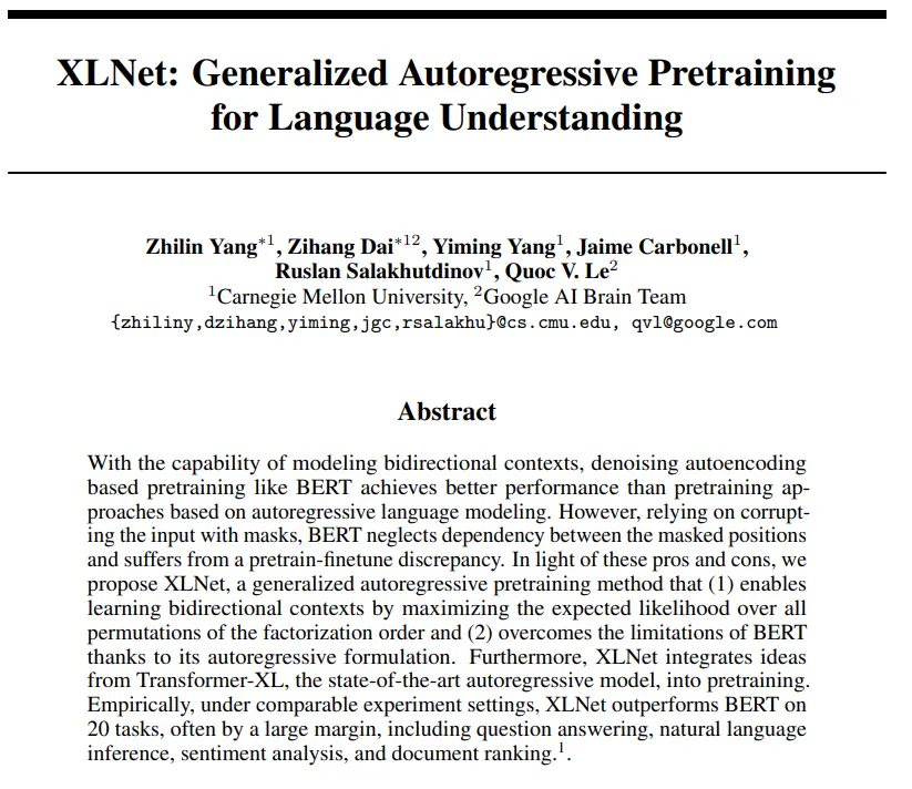
Link to paper: XLNet: Generalized Autoregressive Pretraining for Language Understanding
Quick Summary
XLNet is a novel approach to pretraining language models that combines the advantages of both autoregressive (AR) language models like GPT and autoencoding (AE) models like BERT, while avoiding their limitations.
The key innovation of XLNet is its permutation Language Modeling objective. Rather than using a fixed left-to-right order like traditional autoregressive models, XLNet maximizes the expected log likelihood over all possible permutations of the factorization order for a sequence. This allows each token to effectively see context from both directions while maintaining the autoregressive property.
XLNet addresses two key limitations of BERT:
- It eliminates the independence assumption BERT makes during training (where masked tokens are predicted independently)
- It avoids the pretrain-finetune discrepancy caused by the artificial [MASK] tokens used in BERT
Key architectural components include:
- A two-stream attention mechanism that creates separate content and query streams to enable target-aware predictions
- Integration of Transformer-XL for better handling of long sequences
- Relative positional encodings and relative segment encodings for improved generalization
In empirical evaluations, XLNet outperforms BERT on 20 tasks including question answering, natural language inference, sentiment analysis, and document ranking, often by substantial margins.
It’s hard to break this paper down into a problem and solution segment, As the broader idea was “Both Auto-regressive (Decoder only) & Auto-Encoding (Encoder Only) have their pros and cons, but how do we bring the best of both worlds together”. This is not an easy paper by a long shot. I will try my best to explain it as well as I can.
First we need to understand the pros and cons of AR & AE models as identified by the authors
AE Pros & Cons
Pros:
- It is bidirectional by nature, so it can understand information from both direction
Cons:
-
Independence Assumption: BERT assumes all masked tokens are predicted independently of each other. For the phrase “New York,” if both words are masked, BERT doesn’t use its prediction for “New” to help it predict “York”.
-
Pretrain-Finetune Discrepancy: The artificial
[MASK]symbol used during pre-training is absent during fine-tuning, creating a mismatch that can affect performance.
AR Pros & Cons
Pros:
- Captures the sequential nature of natural language, i.e one word comes after the other.
Cons:
- It is unidirectional, meaning it can only process context from one direction (either left-to-right or right-to-left), which is a disadvantage for many downstream tasks. For example classification
To address the cons of BERT it uses an AR model, and to make it bidirectional. The authors introduce a new idea called Permutation Language Modeling objective.
In this instead of training our models in sequential form 1,2,3,4 and so on. It is instead trained on all possible permutations of the sequence. For example 4,2,1,3/2,4,3,1/1,4,2,3 and many more. Now it is a common source of confusion that the data it self is scrambled. But there is no augmentation done in the data or position encoding side. The embeddings themselves and their positions remain the same.
Instead the attention values are masked. Let us understand how.
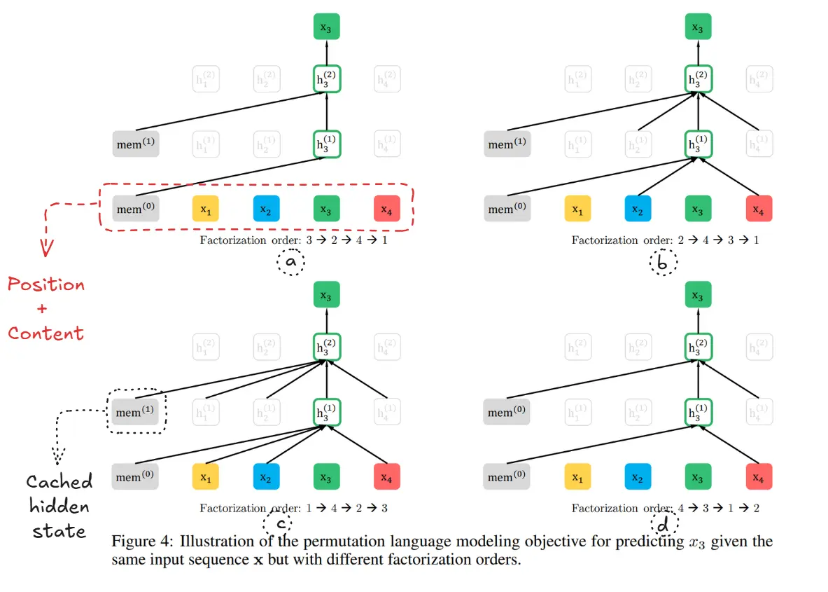 Modified from source
This looks extremely convoluted, I know!! But let’s go through it one by one.
To understand how masking achieves this, let’s look at the image below, which shows how the model predicts the token at position 3 (x₃) under different factorization (prediction) orders.
This looks complex, but the logic is simple: a token can only see other tokens that come earlier in the random permutation order.
-
In panel (a), the order is 3 → 2 → 4 → 1. Since x₃ is the first token to be predicted, its context is empty.
-
In panel (b), the order is 2 → 4 → 3 → 1. Here, x₃ is the third token to be predicted, so it can see the context from the first two predicted tokens, x₂ and x₄.
By doing this over and over with random orders, the model learns that any token can be surrounded by any other token, forcing it to learn a rich, bidirectional understanding of the language.
P.S. mem here is the cached hidden state from the previous segment, an idea inspired by Transformer-XL
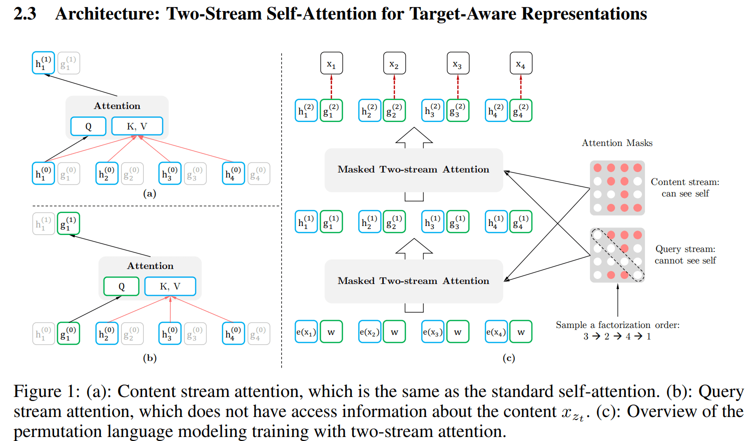
The permutation objective creates a challenge: To predict a token at a target position, the model needs to know the position, but it cannot know the content of the token at that position (otherwise, it would just copy it). A standard Transformer can’t do this, as its hidden state at any position always contains both content and position information.
To solve this, XLNet introduces a Two-Stream Self-Attention mechanism.
Content Stream h (The Memory)
This is the standard Transformer representation. It encodes both the content and position of a token. Its job is to serve as the rich context, or “memory,” that other tokens can attend to. In the image, this is what the nodes labeled h represent.
Query Stream g (The Predictor)
This is a special representation that only has access to the target position, not its content. Its entire purpose is to gather information from the Content Stream of its context tokens to make a prediction for the target position. In the image, this is what the nodes labeled g represent.
In simple terms, for each token being predicted, the Query Stream g asks the question, and the Content Stream h of the other tokens provides the answer. At the final layer, the output of the Query Stream is used to predict the word. During fine-tuning, the query stream is discarded, and we use the powerful, bidirectionally-trained Content Stream for downstream tasks.
Megatron
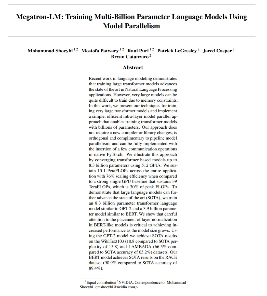
Link to paper: Megatron-LM: Training Multi-Billion Parameter Language Models Using Model Parallelism
Quick Summary
The Megatron-LM paper presents an approach for training extremely large language models using model parallelism that enables training transformer models with billions of parameters. Let me explain the key aspects of this work:
Core Innovation: Simple and Efficient Model Parallelism
The authors implement a simple but effective model parallel approach where they split transformer layers across multiple GPUs in a way that minimizes communication overhead. They do this through:
-
Intra-layer model parallelism: Rather than splitting entire layers across GPUs (pipeline parallelism), they split individual operations within transformer layers.
-
Strategic tensor partitioning: Matrices in transformer layers are partitioned along specific dimensions to minimize communication:
- In the MLP blocks, the first GEMM is split column-wise and the second GEMM is split row-wise
- In self-attention, they partition across attention heads, allowing each GPU to process different attention heads
-
Communication optimization: They carefully place all-reduce operations to minimize the number of synchronization points needed between GPUs.
-
Duplicate computation: Instead of communicating for small operations like dropout or layer normalization, they duplicate these computations across GPUs.
Scaling Achievements
- They established a strong baseline by training a 1.2 billion parameter model on a single GPU that achieves 39 TeraFLOPs (30% of theoretical peak)
- They scaled to an 8.3 billion parameter model using 512 GPUs with 8-way model parallelism and 64-way data parallelism
- They achieved 15.1 PetaFLOPs sustained performance with 76% scaling efficiency compared to the single GPU case
Architecture Innovation for BERT Models
The authors discovered that the standard BERT architecture suffers from degradation when scaled beyond the BERT-Large size. They fixed this by rearranging the layer normalization and residual connections in the architecture, enabling larger BERT models to achieve consistently better results.
Results
Their models achieved state-of-the-art results on:
- WikiText103 (10.8 perplexity vs previous SOTA of 15.8)
- LAMBADA (66.5% accuracy vs previous SOTA of 63.2%)
- RACE dataset (90.9% accuracy vs previous SOTA of 89.4%)
The paper demonstrates that with the right implementation approach, training multi-billion parameter language models is feasible, and these larger models lead to superior performance on a wide range of NLP tasks.
This is a great time to talk about data, model and pipeline paralism and how massively large LLMs are trained across GPUs, Because that is what essential the NVIDIA team did with megatron and shared how they did it!
Obviously Parallel training of huge models on large clusters is a MEGA topic, and we can write books on it. (There are companies and books made on it). So my objective here will be to introduce you to the various concepts of model parallalism, going a bit overboard on what was done in megatron too (for brevity’s sake)
Let us start with the idea of megatron training and we can build on top of that
note: the paper talks about two main ideas, training & how they improved performance on BERT. We will only focus on training in this blog. If you are curious about BERT modifications. Check out the paper!
Now to be complete, We also need to talk about how we can calculate the amount of VRAM required before we start with distributed training. Lest you get too many or too less GPU (Compute is extremely expensive, so we gotta be mindful of what we have)
These are the rough GPU memory requirements:
- FP16 parameter ~ 2 bytes
- FP16 gradient ~ 2 bytes
- FP32 optimizer state ~ 8 bytes based on the Adam optimizers
- FP32 copy of parameter ~ 4 bytes (needed for the optimizer apply (OA) operation)
- FP32 copy of gradient ~ 4 bytes (needed for the OA operation)
Even for a relatively small DL model with 10 billion parameters, it can require at least 200GB of memory, which is much larger than the typical GPU memory (for example, NVIDIA A100 with 40GB/80GB memory and V100 with 16/32 GB) available on a single GPU. Note that on top of the memory requirements for model and optimizer states, there are other memory consumers such as activations generated in the forward pass. The memory required can be a lot greater than 200GB. (Taken from sagemaker AWS documentation)
If you want to understand the memory better I will recommend the following blogs:
- A Gentle Introduction to 8-bit Matrix Multiplication for transformers
- BFloat16: The secret to high performance on Cloud TPUs
Some Misc blogs I found while researching the GPU memory problem:
- HF has a good estimator.
- Calculate it yourself!
- How to build you own machine.
- What hardware you should be getting for Deep Learning.
The following blogs and articles were insanely helpful, While writing the below section:
- This blog gave a great TL;DR with pseudocode (The code in this section has been taken/inspired from here)
- Great overview documentation by HF.
- AWS Documentationhad some nice animations with practical code that helped me understand stuff.
- This blog acted as an awesome glossary and gave good summaries of the ideas.
Naive Parallalism
Naive Model Prallelism, is well… naive and straightforward. Here you just cut the layers of a large model. And put it in different GPUs sequentially.
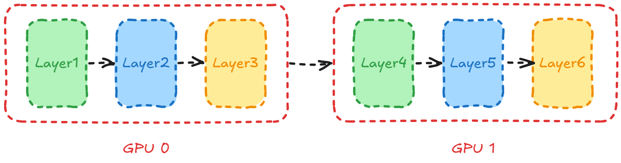 Inspired from here
The implementation is simple as well, you just keep changing the device using .to(), But there are a few problems. The first one being, when the data travels from layer 0 upto layer 3. It is pretty fast as they are in the same device, but when it needs to go to layer 4, this introduced a computational overhead. If both the GPUs are not in the same machine, this will make it very slow.
Another problem is, even though we have 2 devices, while the data is being transfered from layer1 to layer3. The other GPUs remain idle. To fix these problems, the idea of pipeline parallelism was introduced.
# Define model portions
model_part1 = nn.Sequential(layer1, layer2).to('cuda:0')
model_part2 = nn.Sequential(layer3, layer4).to('cuda:1')

# Forward pass
def forward(x):
    x = model_part1(x)
    x = x.to('cuda:1')
    return model_part2(x)
Code taken from here
Pipeline Parallelism
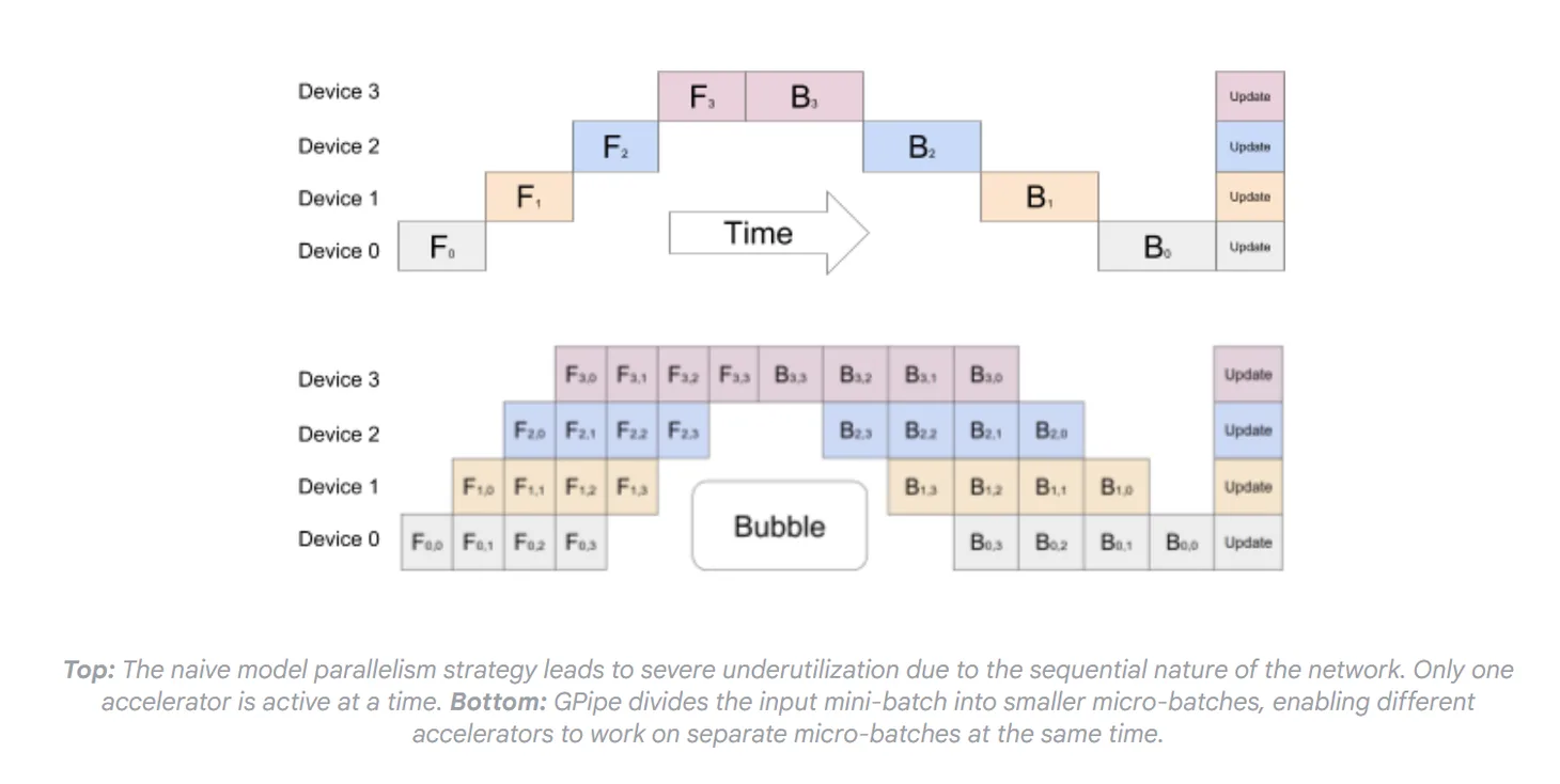
Piepline Parallelism is very similar to Naive MP, We the models split in this too. But to solve the idling problem. The data is sent in mini batches. So each GPU has access to some part of the data and they work somewhat concurrently.
There is an obvious bubble present though, that happens when one GPU is waiting for the gradients to do backprop. In practice, an ideal size of batch along with numbers of GPU is calculated so when one forward pass is completed, mini batch of calculated results keep coming back.
# Define stages
stage1 = nn.Sequential(layer1, layer2).to('cuda:0')
stage2 = nn.Sequential(layer3, layer4).to('cuda:1')

# Pipeline forward
def pipeline_forward(batches):
    for i, batch in enumerate(batches):
        x = stage1(batch)
        x = x.to('cuda:1')
        if i > 0:
            yield stage2(prev_x)
        prev_x = x
    yield stage2(prev_x)
Code taken from here
Data Parallelism
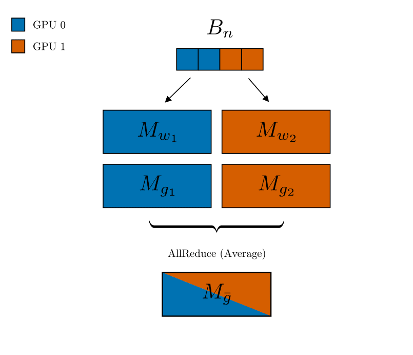
This is another simple method of parallelism. Each device has a full copy of the model, and the data is split between them. And at the end the gradients are synchronized together.
# On each device
for batch in dataloader:
    outputs = model(batch)
    loss = criterion(outputs, targets)
    loss.backward()

    # Synchronize gradients across devices
    all_reduce(model.parameters.grad)

    optimizer.step()
Code taken from here
Tensor Parallelism
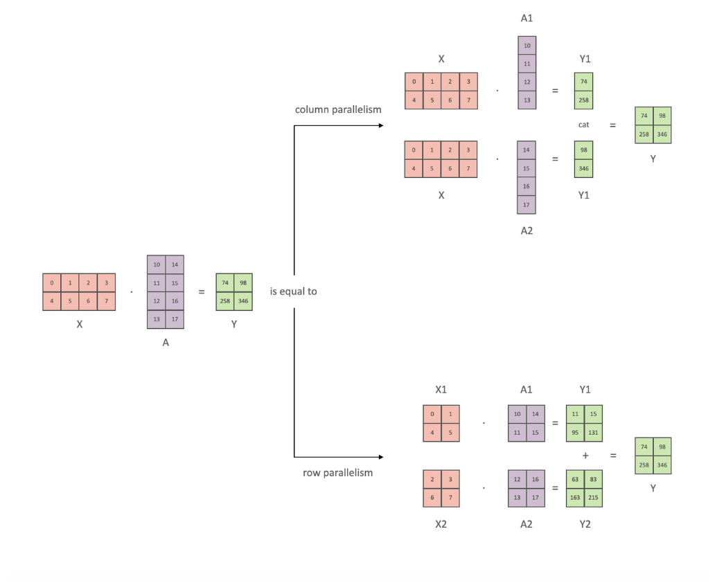
This is the kind of parallelism first introuduce by the megatron paper.
This is a great read on the topic as well github comment.
In this you partition the individual tensors (weights, activations) across devices. And each device computes a portion of the tensor.
This was beautifully explained by the paper, Imagine you have to do an operation (as shown in the above image). We can simply break the matrix and compute it in different devices and put it back together.
Parallelizing the MLP Block
An MLP block contains two linear layers. The first is a GEMM (GEneral Matrix Multiply) followed by a GeLU nonlinearity:
\[Y = \text{GeLU}(XA)\]To parallelize this across two GPUs, the authors split the weight matrix $A$ column-wise: $A = [A_1, A_2]$. The input $X$ is fed to both GPUs, and each computes its part of the operation:
\[[Y_1, Y_2] = [\text{GeLU}(XA_1), \text{GeLU}(XA_2)]\]This is efficient because the GeLU activation can be applied independently on each GPU without any communication.
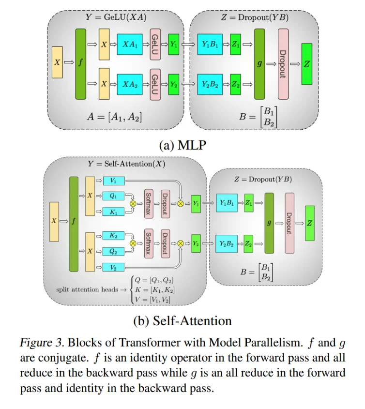
The second linear layer in the MLP block involves another GEMM, $Z = YB$. To make this work, the second weight matrix $B$ is split row-wise:
\[B = \begin{bmatrix} B_1 \\ B_2 \end{bmatrix}\]Each GPU then computes its part, and the results are summed up using an all-reduce operation across the GPUs. This all-reduce is the only communication needed in the forward pass for the MLP block.
Parallelizing the Self-Attention Block
The same principle is applied to the self-attention mechanism. The large weight matrices for Query, Key, and Value ($W_Q, W_K, W_V$) are split column-wise across the GPUs, partitioned by the number of attention heads. Each GPU can compute its share of attention heads independently.
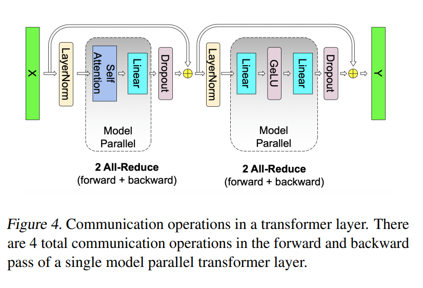
Just like in the MLP block, the output linear layer is split row-wise, and a single all-reduce operation synchronizes the results at the end.
The key takeaway is that this method cleverly arranges the matrix splits so that a full Transformer layer only requires two all-reduce operations in the forward pass (one for the MLP, one for attention) and two in the backward pass. This minimizes communication overhead and leads to excellent scaling efficiency.
# Simplified tensor parallel linear layer
class TPLinear(nn.Module):
    def __init__(self, in_features, out_features, n_devices):
        super().__init__()
        self.weight = nn.Parameter(torch.randn(out_features // n_devices, in_features))

    def forward(self, x):
        local_out = F.linear(x, self.weight)Z
        return all_gather(local_out)
Code taken from here
2d parallalism & 3d parallalism
I mentioned it here to keep you aware of these ideas, we will discuss in depth about them later on. But for now a simple deifition is enough.
- 2d parallism -> When you use two of the techniques described above together.
- 3d parallism -> following the above definition when you use 3 of the above described techniques together it’s called 3d parallism.
There is also ZeRO but we will talk about it when we get to that section.
For a deeper dive into how to implement each and use them in your application, check out the documentation by the PyTorch Team.
Additionally I will recommend checking these two phenomenol blogs by an engineer at Anthropic.
The code behind Megatron-LM
Sparse Attention Patterns
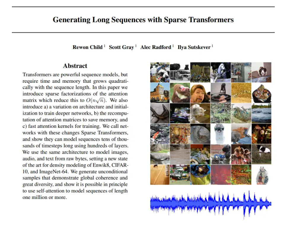
Link to paper: Generating Long Sequences with Sparse Transformers
- Reduced computational complexity for long sequences
Quick Summary
This 2019 paper by Rewon Child, Scott Gray, Alec Radford, and Ilya Sutskever from OpenAI introduces Sparse Transformers, an architectural innovation that makes Transformers more efficient for modeling very long sequences.
Key innovations:
- Introduces sparse factorizations of the attention matrix that reduce computational complexity from O(n²) to O(n√n)
- Proposes architectural modifications to train deeper networks
- Implements memory-efficient recomputation of attention matrices
- Develops fast attention kernels for training
The authors demonstrate that Sparse Transformers can effectively model sequences of tens of thousands of timesteps using hundreds of layers. They apply the same architecture to model images, audio, and text from raw bytes, achieving state-of-the-art results on density modeling tasks for Enwik8, CIFAR-10, and ImageNet-64. Notably, they show it’s possible to use self-attention to model sequences of length one million or more.
Problem
Transformers are awesome, and we all love them (otherwise, you wouldn’t be reading such a huge blog on the topic). But they face one big issue: the self-attention calculation has a quadratic time and memory complexity, which becomes impractical for very long sequences.
Solution
The authors introduce sparse factorization methods to the attention mechanism, reducing its complexity to $O(N\sqrt{N})$. They additionally introduce fast custom kernels and a recomputation method (gradient checkpointing) to save memory.
The following blogs helped me immensely while writing this section:
- Questioning the authors
- Attention? Attention!
- The original blog post by OpenAI
The Cost of Full Attention
If you’ve read this far, I am going to assume you have a fair bit of knowledge about computer science. One of the earliest ideas talked about in CS101 is Big O notation. So let’s quickly calculate the complexity of self-attention.
The self-attention mechanism can be expressed as:
\[\text{Attention}(Q, K, V) = \text{Softmax}\left(\frac{QK^T}{\sqrt{d_k}}\right)V\]Let’s break down the computational complexity step-by-step for a sequence of length $N$:
- Computing $QK^T$: The multiplication of a $[N \times d_k]$ matrix ($Q$) with a $[d_k \times N]$ matrix ($K^T$) results in an $[N \times N]$ attention matrix. The complexity is $O(N^2 \cdot d_k)$.
- Scaling and Softmax: These are element-wise operations on the $[N \times N]$ matrix, so their complexity is $O(N^2)$.
- Multiplying with V: Multiplying the $[N \times N]$ attention matrix with the $[N \times d_v]$ value matrix ($V$) has a complexity of $O(N^2 \cdot d_v)$.
Since the hidden dimensions $d_k$ and $d_v$ are considered constants with respect to the sequence length, the dominant factor is $N^2$. The overall complexity of self-attention is:
\[O(N^2)\]This quadratic cost is computationally expensive for large $N$. This is where Sparse Attention comes in, reducing the complexity to a more manageable $O(N\sqrt{N})$.
Building the Sparse Patterns
The objective of this blog is to help you believe you could have come up with these ideas on your own. So let’s begin by understanding the rationale of the researchers. By visualizing the attention patterns of a deep, fully-trained Transformer, they noticed some recurring themes.
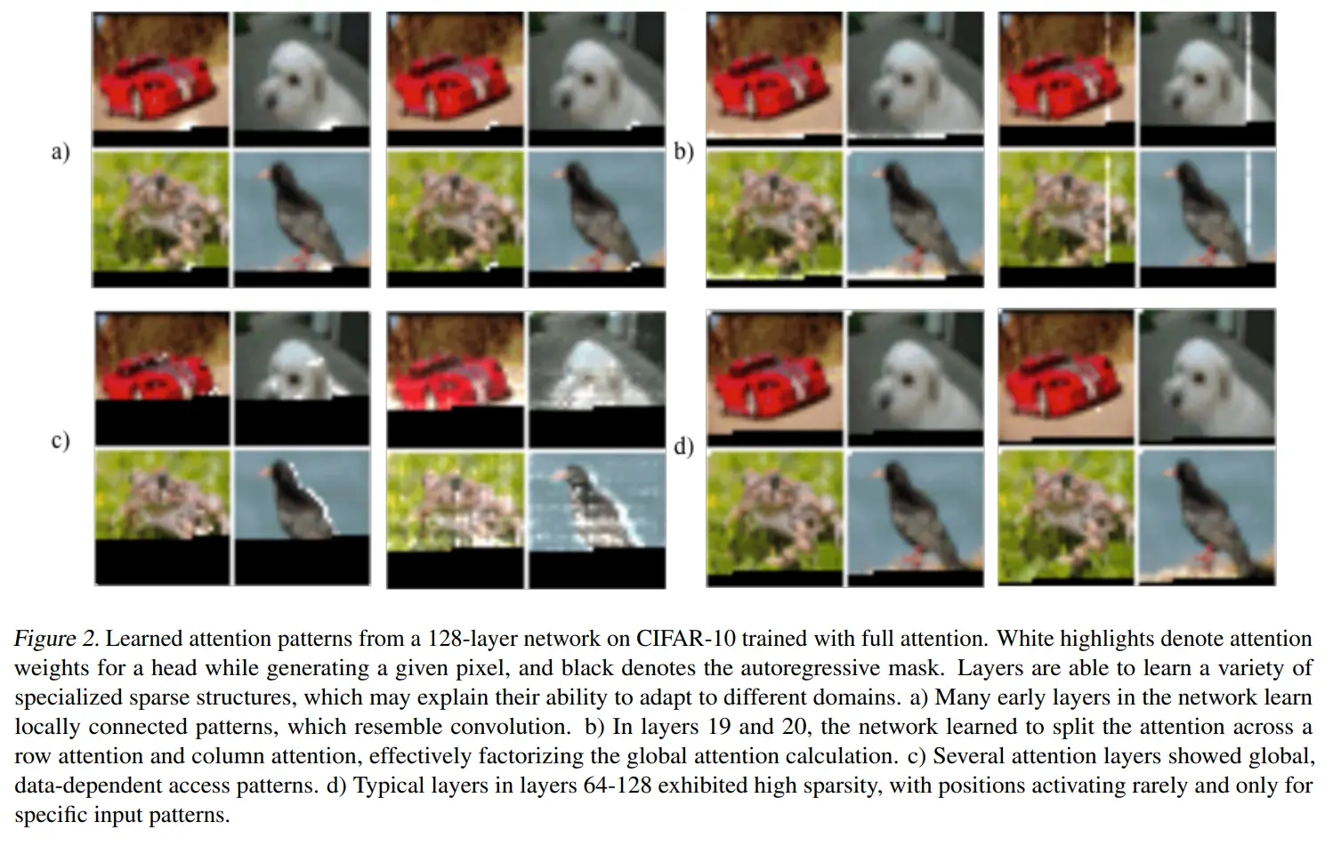 Image taken from the paper, Figure 2
a) Many early layers learned local patterns, resembling convolutions.
b) Some layers learned to attend to entire rows and columns, effectively factorizing the attention.
c) Deeper layers showed global, data-dependent patterns.
d) Surprisingly, the deepest layers exhibited high sparsity, with positions activating rarely.
From these observations, we get a sense of the useful patterns: we need something local, something that can access information globally, and perhaps something in between, like a stride.
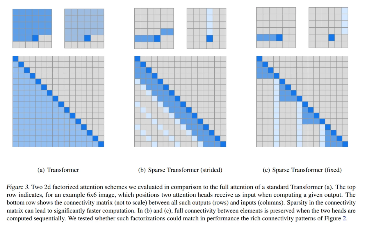 Image taken from the paper, Figure 3
This image might look daunting, but it’s quite simple if we break it down. Let’s quickly clarify the two rows of images. The top row shows the perspective of a single output element (the dark blue square) and which input elements (the light blue squares) it can attend to. The bottom row provides a holistic view of the entire sequence’s connectivity matrix.
Now, let’s look at the patterns:
(b) Strided Attention
This pattern combines two kinds of attention. One head focuses on a local window of nearby positions. For example, the i-th position might only attend to keys from i-w to i, where w is the window size. The other head focuses on more global interactions by having the i-th query attend to every c-th key, where c is the stride. This captures both local context and a coarser, long-range context.
This method works very well for data with a natural periodic structure, like images (where a pixel is related to its neighbors and also to the pixel directly above it). However, it can fail when it comes to text. The reason is that relationships in text are not based on fixed intervals; a word’srelevance to another isn’t determined by a consistent spatial coordinate or stride.
(c) Fixed Attention To solve the problem with text, the authors introduced “fixed attention.” This also uses a local window, but the second head is different. Instead of a stride, it has all future positions attend to a few fixed “summary” locations from previous block.
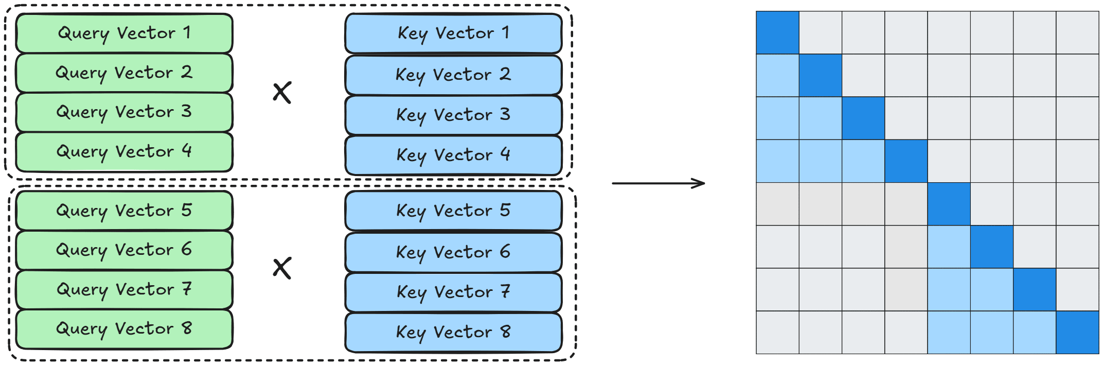 Inspired from here
The local attention creates the block-like structure. This works well but has one big issue: each block only has information from within its own block.
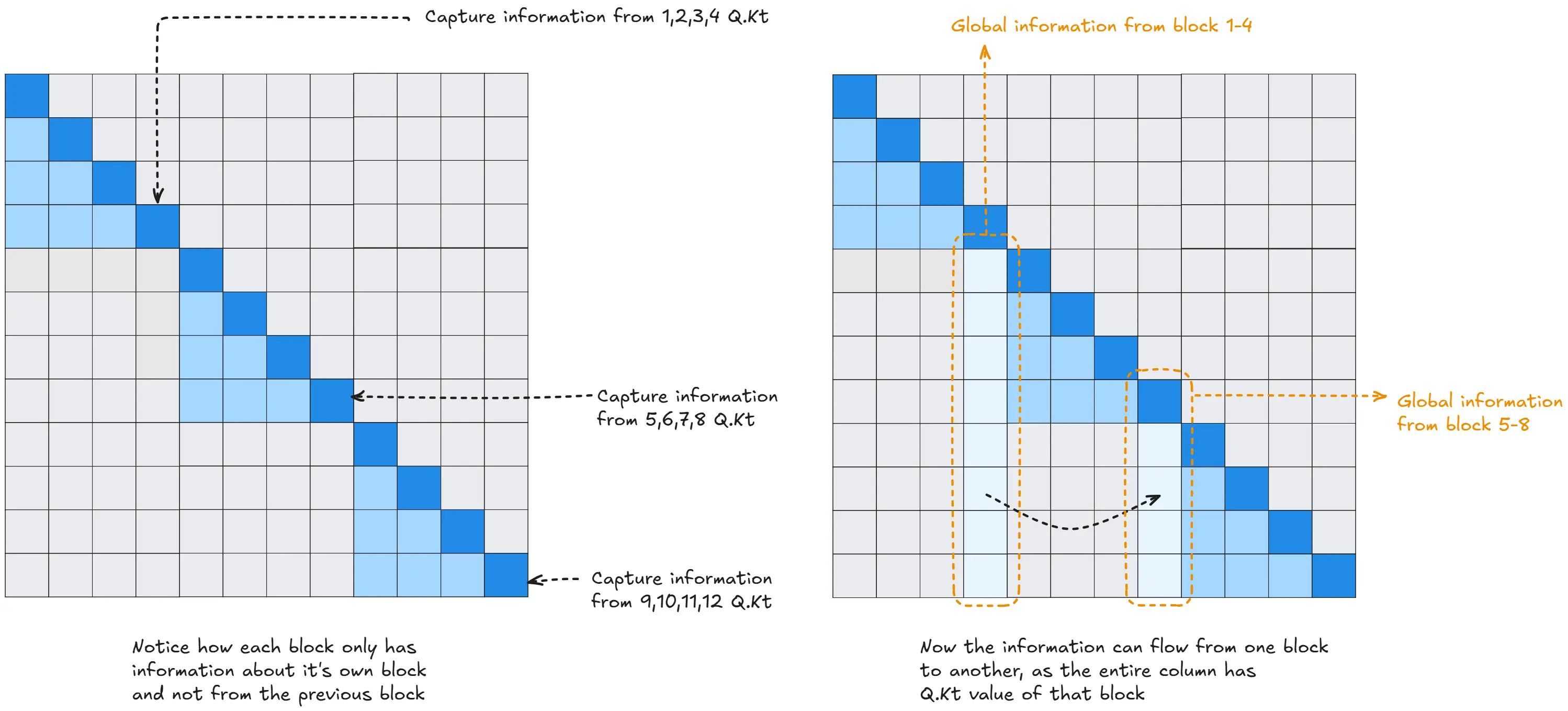 Inspired from here
The fixed summary positions act as “global connectors.” Information captured by the end of a block can now flow globally to all subsequent blocks, allowing the model to connect ideas across the entire sequence.
Calculating the Complexity of Sparse Attention
These sparse patterns significantly reduce the computational cost. Let’s see how, using the formulas from the paper.
In the strided case, each query attends to a local window of size $w$ and roughly $N/c$ strided positions, where $c$ is the stride. The total cost for $N$ queries is:
\[N \left( w + \frac{N}{c} \right) \sim O(N\sqrt{N}), \quad \text{if } c = \sqrt{N}\]In the fixed case, the sequence is split into blocks of length $l$. Each query attends to at most $l$ local positions and $c$ summary positions. The total cost for all queries is:
\[N(l+c) \sim O(N\sqrt{N}), \quad \text{if } l = \sqrt{N}\]In both cases, by carefully choosing the hyperparameters, we can achieve the desired sub-quadratic complexity of $O(N\sqrt{N})$.
Some other ideas introduced in the paper as stated by the authors include:
• A restructured residual block and weight initialization to improve training of very deep networks • A set of sparse attention kernels which efficiently compute subsets of the attenion matrix • Recomputation of attention weights during the backwards pass to reduce memory usage
If you wish to check out the work done by OpenAI, you can do so here: Sparse Attention Repo. They also open-sourced their work on fast kernels: Blocksparse Repo.
NOTICE: Build first, Write later
This blog is now on a short hiatus, I give my reasons here. I will still continue updating this blog, but not as often. Thank you for reading everything I write.
Comments