
Demystifying Diffusion Models
Diffusion models like Stable Diffusion, Flux, Dall-e etc are an enigma built upon multiple ideas and mathematical breakthroughs. So is the nature of it that most tutorials on the topic are extremely complicated or even when simplified talk a lot about it from a high level perspective.
There is a missing bridge between the beautiful simplification and more low level complex idea. That is the gap I have tried to fix in this blog.
- Starting with the simple idea behind diffusion models
- A full section dedicated to the maths for the curious minds
- Understanding each component and coding it out
Each section of the blog has been influenced by works of pioneering ML practitioners and the link to their blog/video/article is linked in the very beginning of the respective section.
How this Blog is Structured
First we will discuss the very high level idea of diffusion models, understanding how they work. In doing so we will be personifying each component of the whole pipeline.
Once we have a general idea of the pipeline, We will dive into the ML side of those sections.
Many sections of the diffusion model pipeline are mathematics heavy, hence I have added a completely different section for that. Which is included after we understand the ML components. You can understand how diffusion models work (if you believe in some assumptions without looking at the proof) along with the code, without the maths. But I will still recommend going through the mathematical ideas behind it, because they are essential for text to image research.
After Understanding everything, we will code it out. As it is substantially harder to keep the blog to a readable length and maintain it’s quality while giving the entire code for Stable Diffusion, I will link to the exact code (with definition for each function) which can help you train the entire pipeline from scratch.
Inference with Diffusion model deserves an entirely different blog of it’s own, as I hope to finish this blog in a reasonable time. I have added links in the end where you can further learn how to make the best diffusion model art and get better at it.
Let us begin!!
The Genius Artist
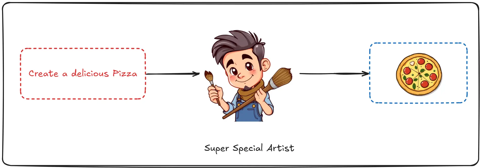 Imagine you have a super special artist friend, whom you tell your ideas and he instantly generates amazing images out of it. Let’s name him Dali.
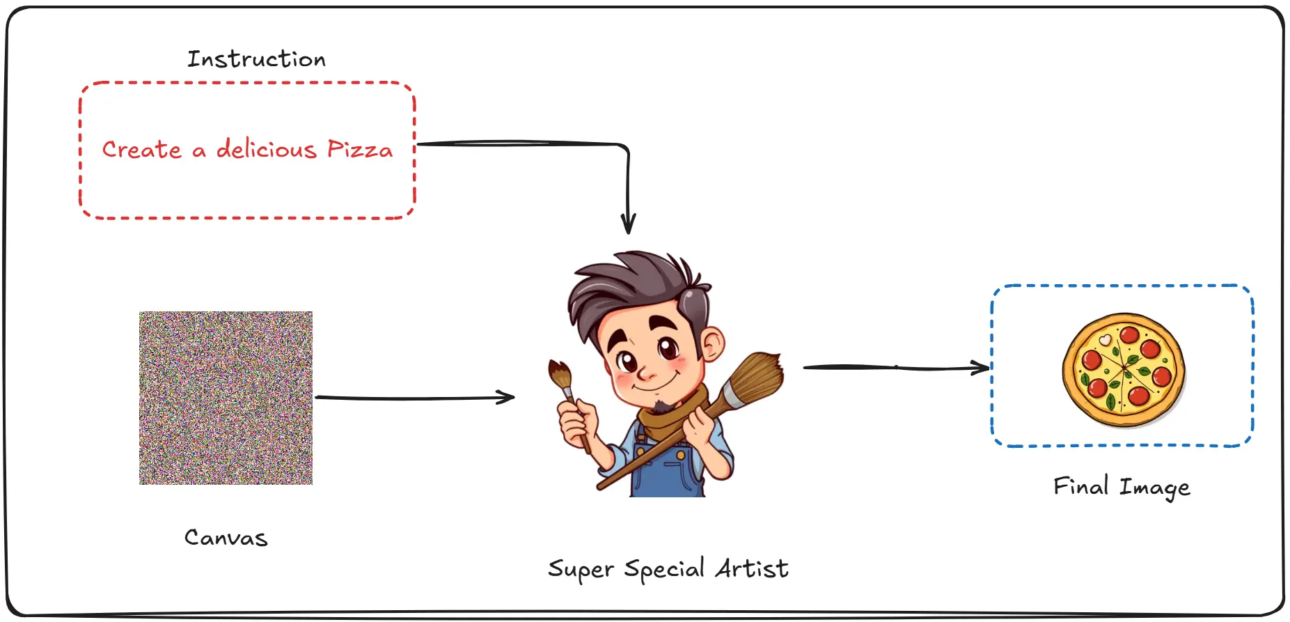 The way Dali starts his work is; He first has a canvas, he then listens to your instructions using which he creates art. (The canvas looks a lot like noise rather than the traditional white, more on this later)
But Dali has a big problem, he cannot make big images, he tells you that he will only create images the size of your hand. This is obviously not desirable. As for practical purposes you may want images the size of a wall, or a poster.
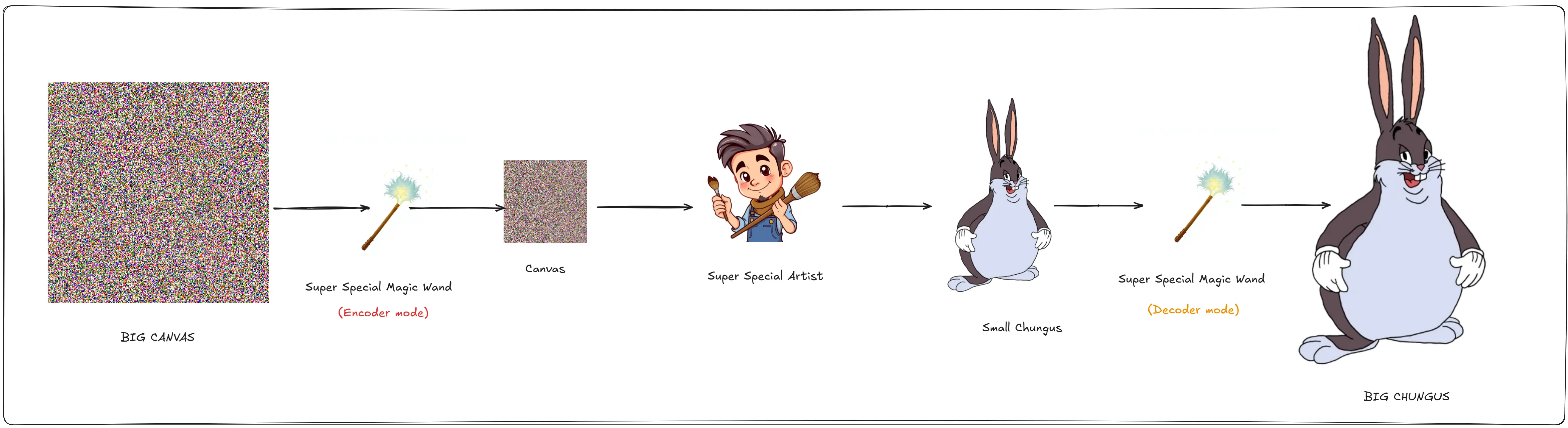
That is when a magic wand falls from the sky, and it has two modes Encoder(Compress size) and Decoder(Enlarge size). That gives you a great idea. You will start with the size of the canvas that you like, Encode it. Give the encoded canvas to Dali, he will make his art, and then you can decode the created art to get it back to the original shape you want.
This works and you are really happy.
But you are curious about how Dali works, so you ask him. “Dali why do you always start with this noisy canvas instead of pure white canvas? and how did you learn to generate so many amazing images?”
Dali is a nice guy, so he tells you about how he started out.
“When I was just a newbie artist. The world was filled with great art. Art so complex that I could not reproduce it, nobody could.”
“Until I found a special wand, which let me add and fix mistakes in a painting.”
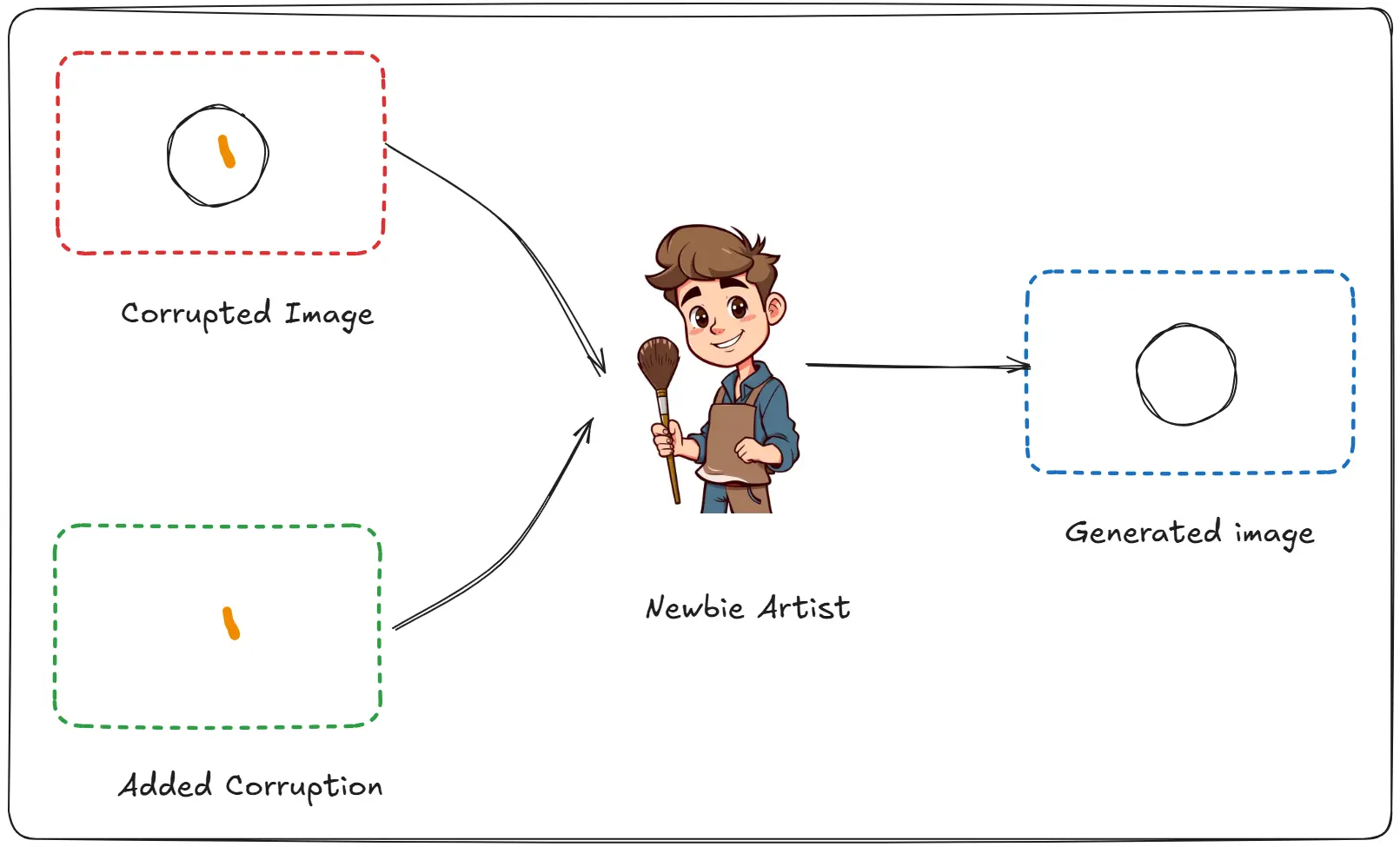
“I would start with an existing artwork, add a bunch of mistakes to it, and using my wand I would reverse them.”
“After a while, I added so many mistakes to the original artwork, that they looked like pure noise. The way my canvas do, and using my special wand. I just gradually found mistakes and removed them. Till I got back the original image.”
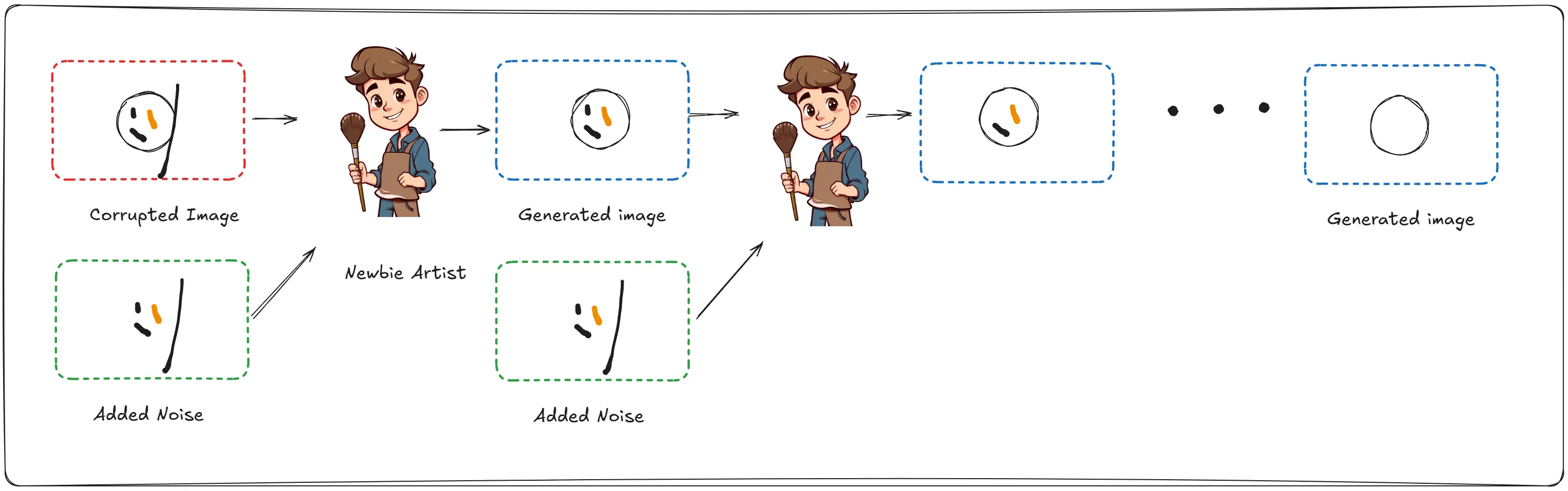
This idea amazes you. But you being you, have quite a question “That sounds amazing, so did you learn what the “full of mistakes” image looks like for all the images in the world? Otherwise how do you know what the final image will be from a noisy image?”
“Great question!!!” Dali responds. “That is what my brothers used to do, They tried to learn the representation of all the images in the world and failed. What I did differently was, instead of learning all the images. I learnt the general idea of different images. For example, instead of learning all the faces. I learnt how a face looks like in general”
Satisfied with his answers you were about to leave, when Dali stops you and asks, “Say friend, that wand of yours truly is magical. It can make my art popular worldwide because everyone can create something of value using it. Will you be kind enough to explain how it works so I can make one for myself.”
You really want to help Dali out, but unfortunately even you do not know how the wand works, as you are about to break the news to him. You are interrupted by a noise, “Gentlemen you wouldn’t happen to have seen a magic wand around now would you? It is an artifact created with great toil and time”
You being the kind soul you are, tell the man that you found it on the street and wish to return it. The man greatly happy with your generosity, wishes to pay you back. You reply with “Thank you, but I do not seek money. It would be nice if you could help my friend Dali out, by explaining how your magic wand works.”
The man curious for what use anyone would have for his magic wand sees around Dali’s studio, and understands that he is a great artist. Happy to help him he says. “My name is Auto, and I shall tell you about my magic wand.”
“There is a special dimension that my grandpappy found, where everything big can be made small, and when we try to get these small things back from this dimension. It turns back big in our world.
That is what the encode command of the wand does, it turns the object into how it would look like in the special dimension.
You can then make changes to the object, And when we do the decode command. It turns it back into this dimension making it big.
I will give you as many wands as you want!!”
Dali is extremely happy, you are happy for your friend, and Auto is happy that he got a new customer.
The end.
Understanding Stable Diffusion
Now that you have a general idea of how these image generation models work, let’s understand each specific component out. Beginning with the U-Net, which predicts the noise. Then moving on to the Scheduler, responsible for removing the predicted noise. After which we will have a look at the different Conditioning like text encoders, ControlNet, LoRA etc. And finally finish by understanding VAEs, which revolutionized diffusion models and is the foundation of high quality image generation.
Also, the respective code in each section is for understanding purposes. If you wish to run the entire pipeline, go to this repo.
Additionally, The below work takes heavy inspiration from the following works:
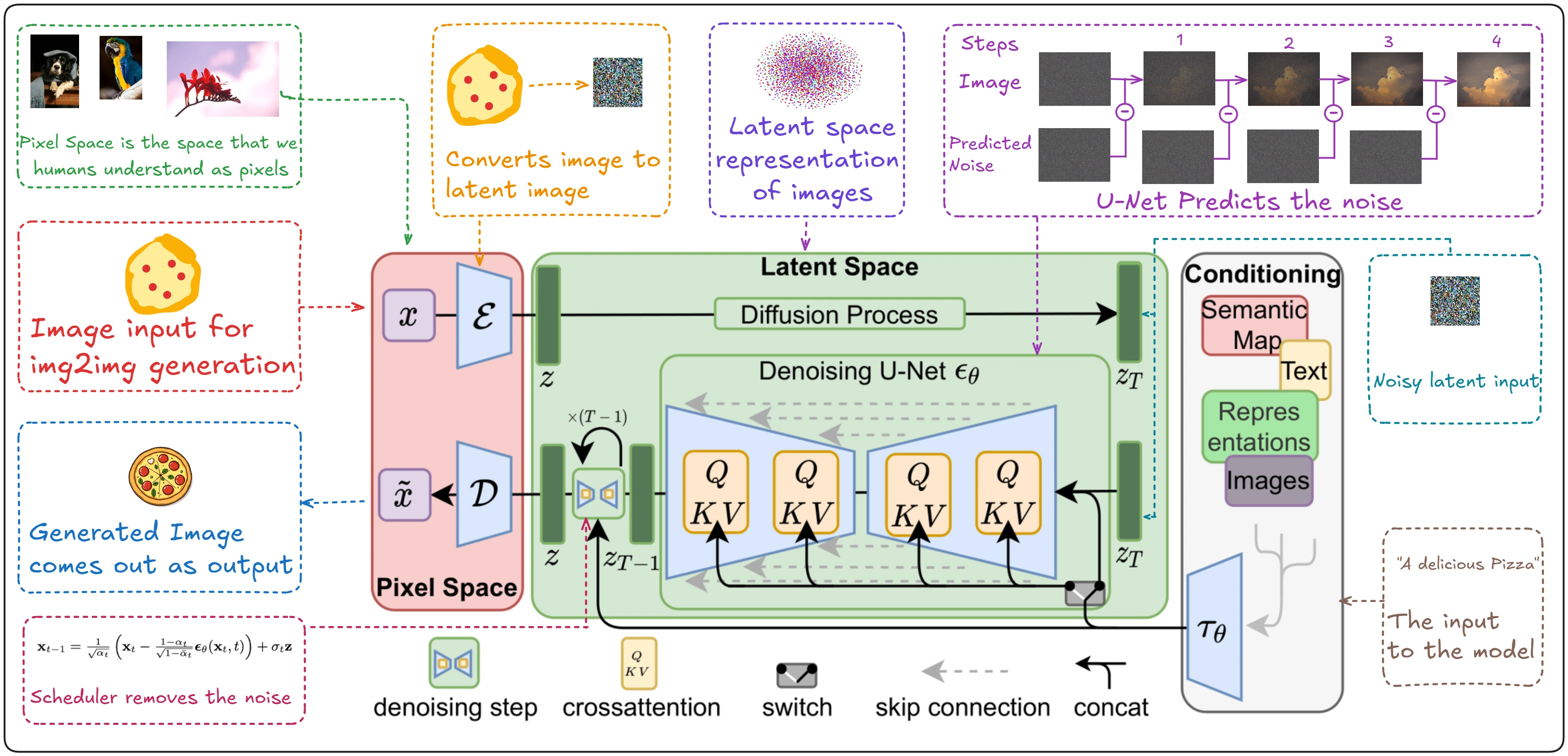
If you look closely you will see how similar both these images are.
The above is an oversimplification and has a few mistakes. But by the end of this blog you will have a complete understanding of how diffusion models work and how the seemingly complex model above, is quite simple.
Dali The Genius Artist (U-Net)
Our genius artist is called a U-Net in ML terms, now if we go back to our story. Dali was responsible for figuring out the noise. The removal and addition of which was done by his magic wand. That is what the U-Net does. It predicts the noise in the image, it DOES NOT REMOVE IT.
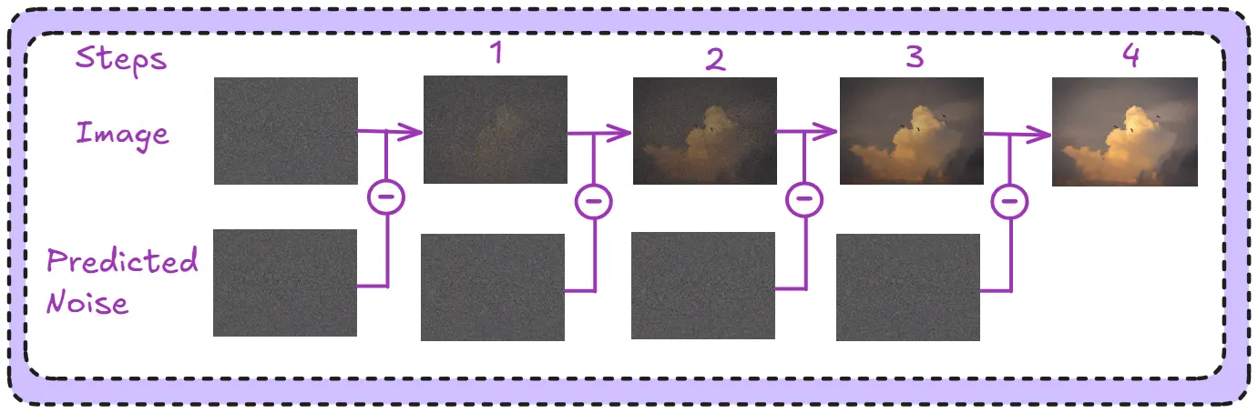
In the above image, the U-Net predicts the noise in a step wise manner. The scheduler is responsible for removing it (indicated by the “-“ sign).
Let’s understand how it works.
You will be surprised to know U-Nets were actually introduced in a medical paper back in 2015. Primarily for the task of image segmentation.
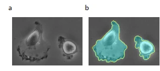
Image taken from the “U-Net: Convolutional Networks for Biomedical Image Segmentation”
The idea behind segmentation is, given an image “a”. Create a map “b” around the objects which needs to be classified in the image.
And the reason these are called U-Nets is because, well the architecture looks like a “U”.
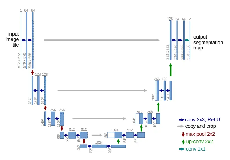
Image taken from the “U-Net: Convolutional Networks for Biomedical Image Segmentation”
This looks quite complicated so let’s break it down with a simpler image.
Also, I will proceed with the assumption you have an understanding of CNNs and how they work. If not, check the misc for a guide to where you can learn more on the topic.
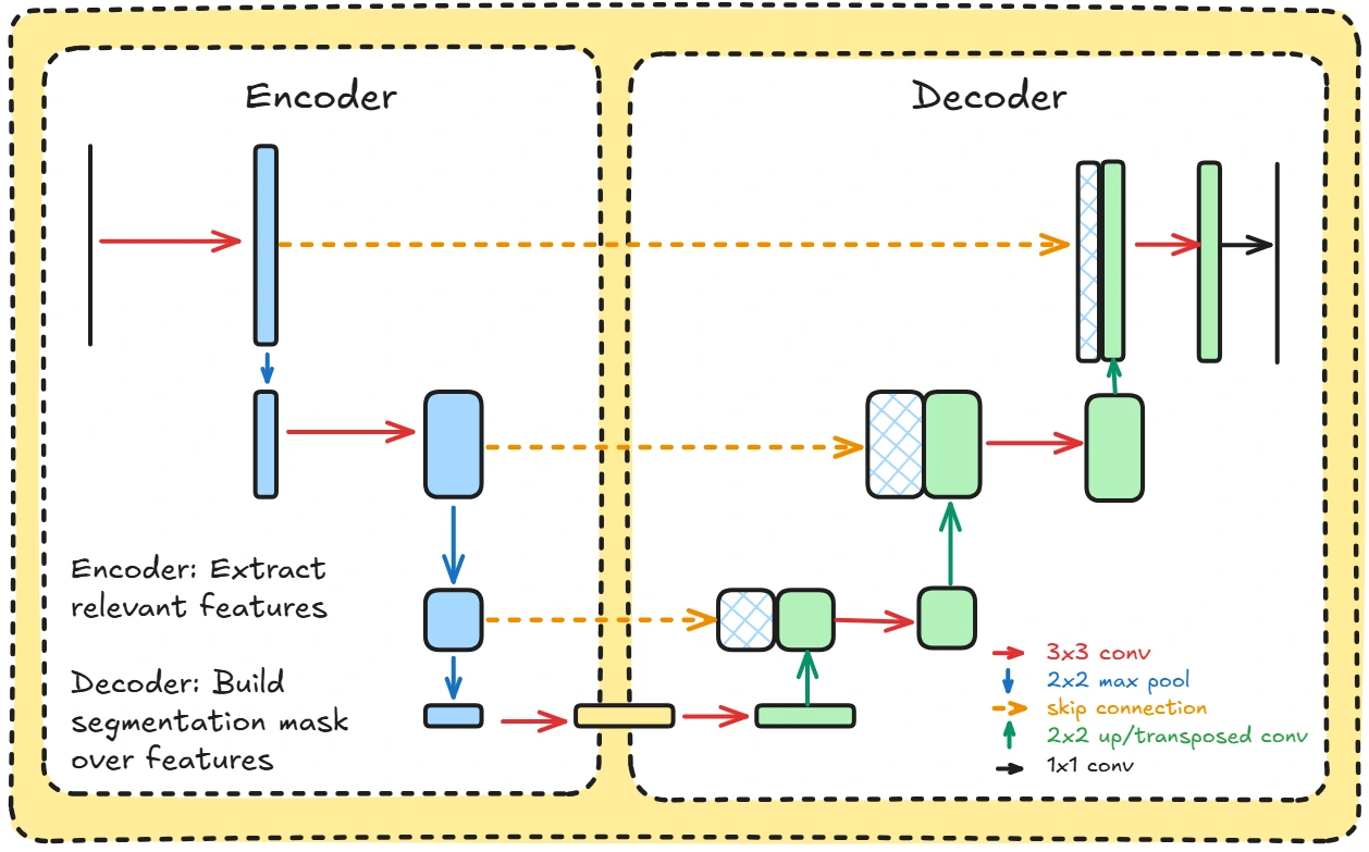
The encoder side does convolutions to extract features from images, then compresses them to only focus on the relevant parts.
The decoder then does transpose convolutions to decode these extracted parts back into the original image size.
To understand it in our context, think instead of segmenting objects, we are segmenting the noise. Trying to find out the particular places where noise is present.
To prevent the U-net from losing important information while down-sampling, skip connections are added. These send the compressed encoded image back to the decoder so they have context from there as well.
Coding the original U-Net
It’s easier to understand when we write it down in code. So let us do that. (We start with coding the original U-Net out first, then add the complexities of the one used in Stable Diffusion later)
class DoubleConv(nn.Module):
    def __init__(self, in_channels, out_channels):
        super().__init__()
        self.double_conv = nn.Sequential(
            nn.Conv2d(in_channels, out_channels, kernel_size=3, padding=1),
            nn.BatchNorm2d(out_channels),
            nn.ReLU(inplace=True),
            nn.Conv2d(out_channels, out_channels, kernel_size=3, padding=1),
            nn.BatchNorm2d(out_channels),
            nn.ReLU(inplace=True)
        )

    def forward(self, x):
        return self.double_conv(x)
This is a simple convolution, This is done to extract relevant features from the image.
class Down(nn.Module):
    def __init__(self, in_channels, out_channels):
        super().__init__()
        self.maxpool_conv = nn.Sequential(
            nn.MaxPool2d(2),
            DoubleConv(in_channels, out_channels)
        )

    def forward(self, x):
        return self.maxpool_conv(x)
A simple Down block, that compresses the size of the image. This makes sure we only focus on the relevant part. Imagine it like this given most images, like pictures of dogs, person in a beach, photo of the moon etc. The most interesting part (the dog, person, moon) usually take up a small part of the image.
class Up(nn.Module):
    def __init__(self, in_channels, out_channels, bilinear=True):
        super().__init__()
        # Choose between two upsampling methods
        if bilinear:
            # Method 1: Simple bilinear interpolation
            # Doubles the spatial dimensions using interpolation
            self.up = nn.Upsample(scale_factor=2, mode='bilinear', align_corners=True)
        else:
            # Method 2: Learnable transposed convolution
            # Doubles spatial dimensions while halving channels
            self.up = nn.ConvTranspose2d(in_channels, in_channels // 2, kernel_size=2, stride=2)

        # Apply two consecutive convolutions after combining features
        self.conv = DoubleConv(in_channels, out_channels)

    def forward(self, x1, x2):
        # Step 1: Upsample the lower resolution feature map (x1)
        x1 = self.up(x1)

        # Step 2: Handle size mismatches between upsampled and skip connection
        # Calculate the difference in height and width
        diff_y = x2.size()[2] - x1.size()[2]  # Height difference
        diff_x = x2.size()[3] - x1.size()[3]  # Width difference

        # Add padding to make sizes match
        # The padding is distributed evenly on both sides
        x1 = F.pad(x1, [diff_x // 2, diff_x - diff_x // 2,
                       diff_y // 2, diff_y - diff_y // 2])

        # Step 3: Combine features from upsampled path and skip connection
        x = torch.cat([x2, x1], dim=1)  # Concatenate along channel dimension

        # Step 4: Process combined features through double convolution
        return self.conv(x)
This is the Up sampling block that helps generate the mask, which is needed for segmentation of the image.
class UNet(nn.Module):
    def __init__(self, num_classes):
        super().__init__()

        # Correct channel progression:
        self.inc = DoubleConv(3, 64)  # Initial convolution

        # Encoder path (feature maps halve, channels double)
        self.down1 = Down(64, 128)    # Output: 128 channels
        self.down2 = Down(128, 256)   # Output: 256 channels
        self.down3 = Down(256, 512)   # Output: 512 channels
        self.down4 = Down(512, 1024)  # Output: 1024 channels

        # Decoder path (feature maps double, channels halve)
        self.up1 = Up(1024, 512)      # Input: 1024 + 512 = 1536 channels
        self.up2 = Up(512, 256)       # Input: 512 + 256 = 768 channels
        self.up3 = Up(256, 128)       # Input: 256 + 128 = 384 channels
        self.up4 = Up(128, 64)        # Input: 128 + 64 = 192 channels

        # Final convolution
        self.outc = nn.Conv2d(64, num_classes, kernel_size=1)

    def forward(self, x):
        # Store encoder outputs for skip connections
        x1 = self.inc(x)         # [B, 64, H, W]
        x2 = self.down1(x1)      # [B, 128, H/2, W/2]
        x3 = self.down2(x2)      # [B, 256, H/4, W/4]
        x4 = self.down3(x3)      # [B, 512, H/8, W/8]
        x5 = self.down4(x4)      # [B, 1024, H/16, W/16]

        # Decoder path with skip connections
        x = self.up1(x5, x4)     # Use skip connection from x4
        x = self.up2(x, x3)      # Use skip connection from x3
        x = self.up3(x, x2)      # Use skip connection from x2
        x = self.up4(x, x1)      # Use skip connection from x1

        # Final 1x1 convolution
        logits = self.outc(x)    # [B, num_classes, H, W]

        return logits
By putting together the Down and Up blocks we have the final U-Net as coded above.
Stable Diffusion U-Net
The Diffusion Model U-Net is quite different. But it follows the same principles as discussed above.
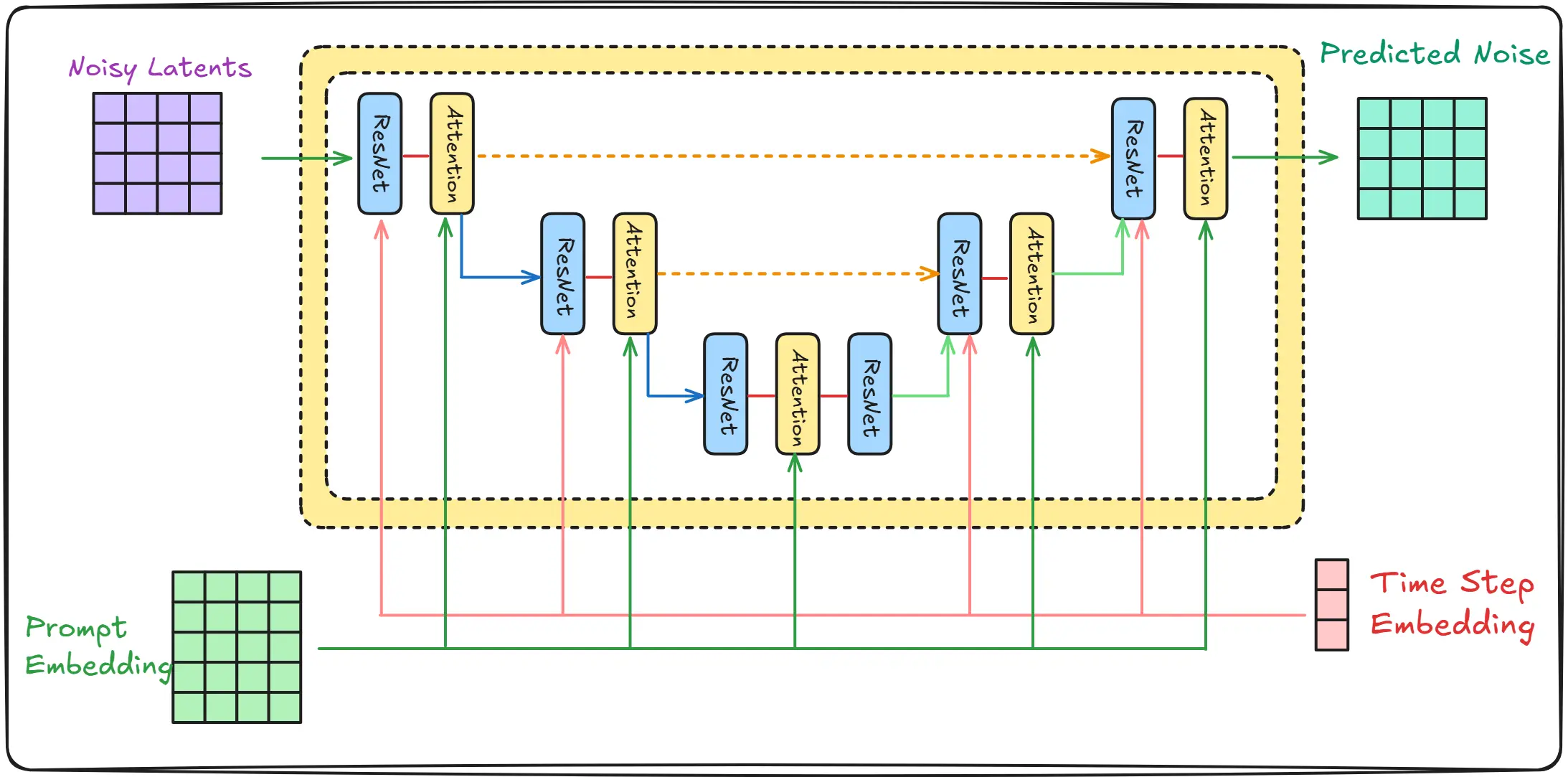
First, let’s understand what goes into this U-Net:
Input Components
- Noisy Latents: The noisy image we’re trying to denoise
- Prompt Embedding: Text information converted into a numerical representation
- Timestep Embedding: Information about which denoising step we’re on
The ResNet and Attention blocks work together in a complementary way to process this information:
ResNet Blocks
These blocks receive three inputs that are combined:
- The main feature path (coming from previous layers)
- The timestep embedding
- The residual skip connection (from earlier in the network)
Inside a ResNet Block (pseudo-code):
# Simplified ResNet block structure
def resnet_block(features, time_embedding, skip_connection):
    # Time embedding projection
    time_features = project_time_embedding(time_embedding)

    # Combine features with time information
    combined = features + time_features

    # Apply convolutions with residual connection
    output = conv1(combined)
    output = activation(output)
    output = conv2(output)

    # Add skip connection
    final = output + skip_connection
    return final
If you are new to ResNets, consider reading more here.
The ResNet blocks are crucial because they:
- Maintain spatial information about the image
- Help the model understand how features should change based on the denoising step
- Prevent vanishing gradients through residual connections
Attention blocks receive:
- The feature maps from ResNet blocks
- The prompt embedding (indirectly through cross-attention)
Inside an attention block (pseudo-code):
# Simplified attention block structure
def attention_block(features, prompt_embedding):
    # Self-attention: Image features attending to themselves
    q, k, v = project_to_qkv(features)
    self_attention = compute_attention(q, k, v)

    # Cross-attention: Image features attending to text
    q_cross = project_query(features)
    k_cross, v_cross = project_kv(prompt_embedding)
    cross_attention = compute_attention(q_cross, k_cross, v_cross)

    # Combine both attention results
    output = self_attention + cross_attention
    return output
To read more about attention, consider reading my blog on the topic here.
The attention blocks are essential because they:
- Help the model focus on relevant parts of the image based on the text prompt
- Allow the model to understand relationships between different parts of the image
- Enable text-image alignment during the generation process
Why This Architecture Works So Well
-
Progressive Refinement
- The U-Net structure allows the model to work at multiple scales
- Early layers capture broad structure
- Middle layers refine details
- Later layers add fine details
-
Information Flow
- ResNet blocks ensure gradient flow and feature preservation
- Attention blocks align image generation with text description
- Skip connections preserve spatial information
-
Controlled Generation
- Timestep embeddings guide the denoising process
- Prompt embeddings guide the semantic content
- Their combination enables precise control over the generation
For example, when generating an image of “a red cat sitting on a blue chair”:
- ResNet blocks handle the basic structure and progressive denoising
-
Attention blocks ensure:
- The cat is actually red
- The chair is actually blue
- The cat is positioned correctly relative to the chair
- Skip connections preserve spatial details throughout the process
Diffusion Transformer (DiT)
There’s another architecture that’s becoming increasingly popular - the Diffusion Transformer (DiT). Think of it as giving Dali a different kind of artistic training, one that’s more about seeing the whole canvas at once rather than focusing on different parts separately.
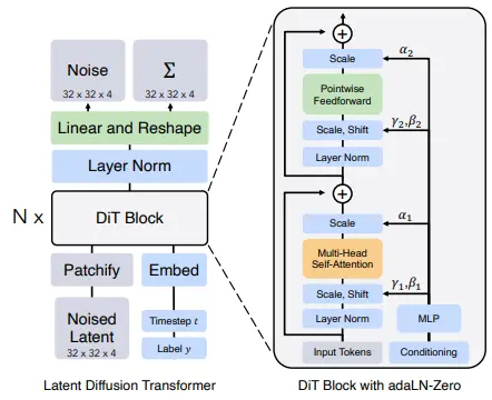
Image taken from “Scalable Diffusion Models with Transformers”
To understand DiTs, let’s first recall what made U-Nets special:
- They look at images at different scales (like an artist looking at both details and the big picture)
- They have skip connections (like keeping notes about earlier versions of the painting)
- They process information in a hierarchical way (working from rough sketch to fine details)
DiTs take a completely different approach. Instead of processing the image in this hierarchical way, they treat the image more like a sequence of patches - imagine cutting up the canvas into small squares and looking at how each square relates to all other squares.
Here’s how it works:
-
Patch Embedding:
- The noisy image is divided into small patches (usually 16×16 pixels)
- Each patch is converted into a sequence of numbers (like translating visual information into a language DiT can understand)
- If this reminds you of how CLIP processes images, you’re spot on!
-
Global Attention:
- Unlike U-Net where each part mainly focuses on its neighbors, in DiT every patch can directly interact with every other patch
- It’s like the artist being able to simultaneously consider how every part of the painting relates to every other part
- This is done through transformer blocks, similar to what powers ChatGPT but adapted for images
-
Time and Prompt Integration:
- The noise level (timestep) is embedded directly into the sequence
- Text prompts are also converted into embeddings and can influence how patches interact
- This creates a unified way for the model to consider all the information at once
The advantages of DiTs are:
- Better at capturing long-range relationships in images (like ensuring consistency across the entire image)
- More flexible in handling different types of inputs
- Often easier to scale up to larger models
But there’s no free lunch - DiTs typically require more computational resources than U-Nets and can be trickier to train. This is why many popular models still use U-Nets or hybrid approaches.
A practical example of DiT’s power is in handling global consistency. Let’s say you’re generating an image of “a symmetrical face”:
- A U-Net might need to work hard to ensure both sides of the face match
- A DiT can more easily maintain symmetry because it’s always looking at the relationship between all parts of the face simultaneously
The future is likely to see more models using DiT architectures or hybrid approaches combining the best of both U-Net and DiT worlds. After all, even great artists can learn new techniques!
Dali’s mistake fixing wand (Scheduler)
A quick note, This part is mostly purely mathematical. And as mentioned earlier, everything is described in greater detail in the maths section.
This here is mostly a quick idea that one will need to understand how scheduler’s work. If you are interested in how these came to be, I urge you to check out the mathematics behind it, because it is quite beautiful.
Also, if at any point during the explanation, it becomes too complex to comprehend. Consider taking a break and continuing later, Each part alone took me weeks to write. Do not assume you can understand it in one sitting, and the idea only becomes simpler as you read more about it.
As mentioned earlier, The U-Net does not remove the noise, it just predicts it. The job of removing it comes down to the scheduler.
Put simply, the scheduler is just a mathematical equation that takes an image & predicted noise. And outputs another image with some noise removed from it. (I am saying images, but actually matrices are passed around)
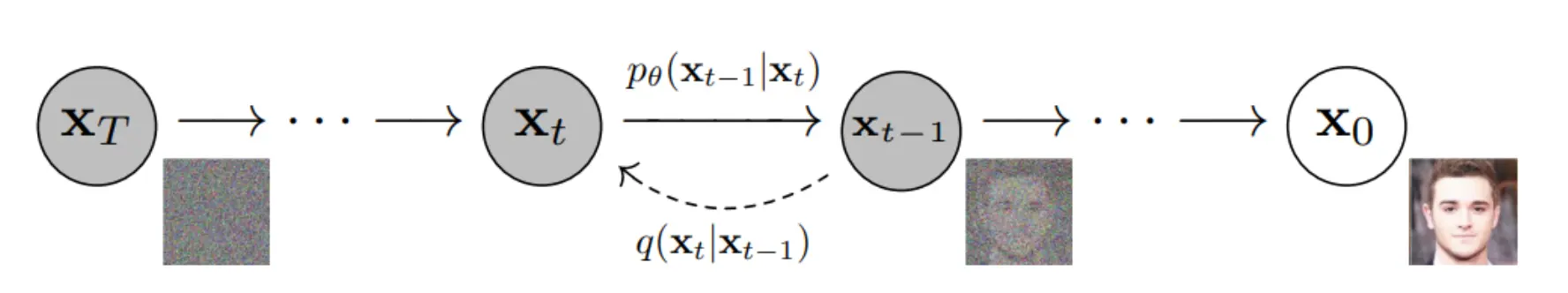
Image taken from “Denoising Diffusion Probabilistic Models”
The above image looks quite complex, But it is really simple if you understand what is going on.
We start with an image and call it $X_0$ we then keep adding noise to it till we have pure Stochastic (Random) Gaussian (Normal Distribution) Noise $X_T$ (A completely noisy image).
\[q(x_t|x_{t-1})\]“The above equation is the conditional probability over the Probability Density Function”
Well wasn’t that a mouthful, don’t worry. I won’t throw such a big sentence at you without explaining what it means.
Let’s again start with our original image $X_0$ and then add a bit of noise to it, this is now $X_1$, then we add more noise to this image and it becomes $X_2$ and we can keep doing this for $t$ steps.
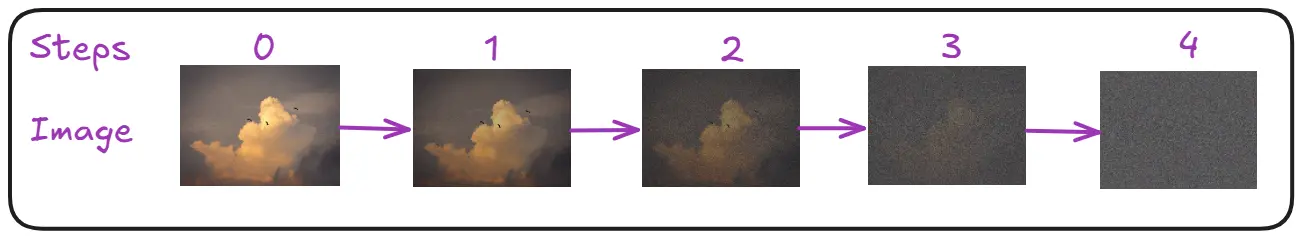
That scary looking equation basically says if we have an image $X_{t-1}$ we can add noise to it and get the image at the next timestep, represented as $X_t$ (This is a slight oversimplification and we dive into greater detail about it in the math section)
So now we have a single image, and we are able to add noise to it.
Note: A simple method I use to keep in mind, whenever an equation like p(A|B) is present. Simply think right to left. Given B, what can be A.
What we want to do is, the reverse process. Take noise and get an image out of it.
You may ask why do we not simply do what we did earlier but the other way around so something like
\[q(X_{t-1}|X_t)\]Well the above is simply not computationally possible (Intractable is the lingo used for it in software world) because we will need to learn how the noise of all the images in the world looks like (remember how in the idea section Dali said his brothers tried to do this and failed)
So we need to learn to approximate it, learn how the images might look like given the noise.
and that is given by the other equation
\[p_\theta(x_{t-1}|x_t)\]Now above I mentioned that we add noise, but never described how.
That is done by this equation
\[q(x_t|x_{t-1}) = \mathcal{N}(x_t; \sqrt{1-\beta_t}x_{t-1}, \beta_t\mathbf{I})\]We already know what the left hand side (LHS) means, lets understand the right hand side (RHS).
The RHS represents a Normal distribution $\mathcal{N}$ with mean $\sqrt{1-\beta_t}x_{t-1}$ and variance $\beta_t\mathbf{I}$, where we sample noise at time $t$ from this distribution to add to our image.
There is one slight problem though, gradually adding noise at different values of t is very computationally expensive.
Using the “nice property” we can make another equation. (Explained and derived in the maths section)
\[q(x_t|x_0) = \mathcal{N}(x_t; \sqrt{\bar{\alpha}_t}x_0, (1-\bar{\alpha}_t)\mathbf{I})\]where \(\alpha_t = 1-\beta_t\) and \(\bar{\alpha}_t = \prod_{i=1}^t \alpha_i\)
($\prod_{i=1}^t \alpha_i$ means the values of alpha multiplied from $1$ to $t$, $\alpha_1 \cdot \alpha_2 \cdot \alpha_3 \cdot … \cdot \alpha_t$)
This equation lets us add noise at any time t just using the original image. This is amazing, why? Because during training it will be very tough to go sequentially from $t=1$ to $t=n$ just to figure out how the noisy image will look like at timestep $n=40$. The above equation saves us from this computational inefficiency.
Note: we have been repeatedly using the term timestep. Funny enough it has nothing to do with time. It is just a name used in convention. We might as well replace it simply with Step or even Count. So do not think timestep with a notion of time. But rather the number of steps.
You need to understand a few more things, the $\beta$ term in the above equation is a variance shedule it basically controls the curve the noise is added into the image.
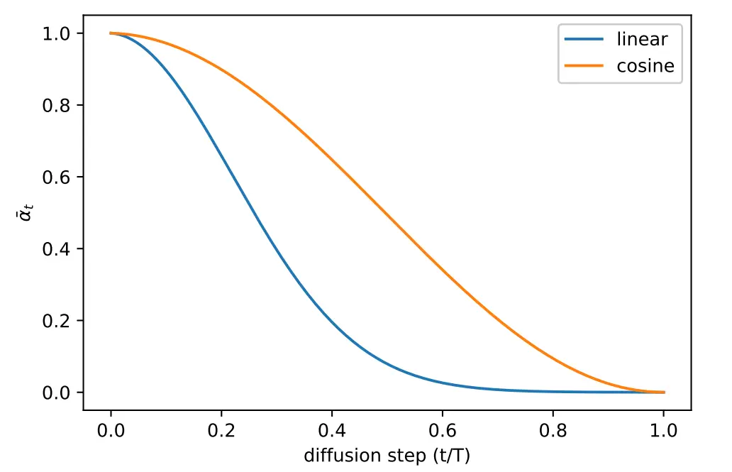
Image taken from “Improved Denoising Diffusion Probabilistic Models”
The above image represents how value of $\beta$ is varied.
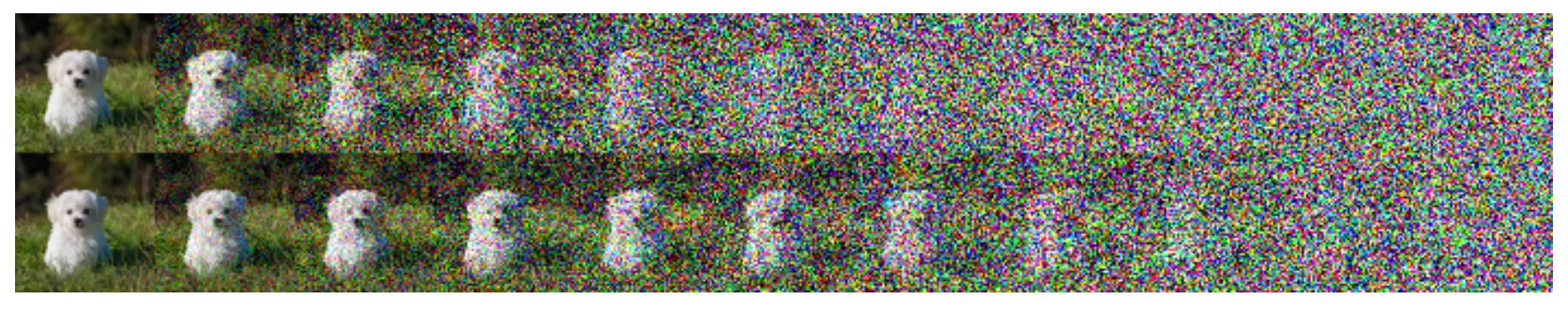
Image taken from “Improved Denoising Diffusion Probabilistic Models”
Top is noise being added by a linear variance scheduler, notice how after only a few steps the image starts looking like complete noise
Bottom is noise being added by a cosine variance scheduler.
Now that we understand how we can add noise to the images & how we can control the different kinds of noise. There is something much more important that we still haven’t talked about, that is. WHY ARE WE DOING THIS and WHY DOES THIS WORK?
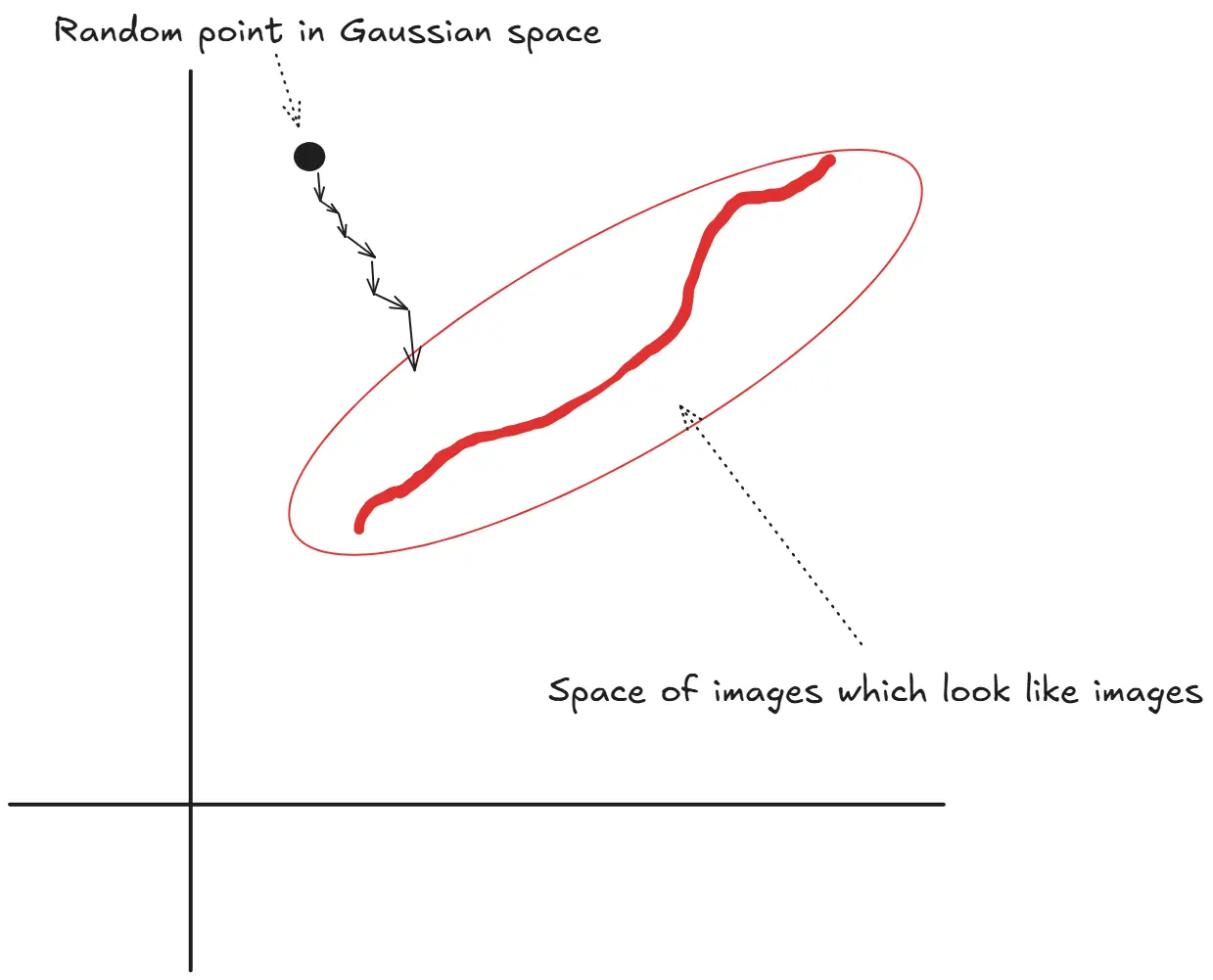
Images that look like images actually lie is a very specific region of all possible images in the world. An easy way to think about it will be like this, most humans only have 2 eyes. But if you are given an infinite space of images, the pictures of humans can have n number of eyes. But you only want the images which has 2. So that significantly limits the space from where you want to get your images.
Hence, initially by adding noise to an image. We are taking it from this very specific space, to the more random gaussian space. (This is done, so we can learn the reverse process. Given any random point in space, get back to this very specific space)
We have been constantly talking about adding Gaussian Noise, but haven’t discussed the reason. So let’s take a minute to understand the rationale behind that as well.
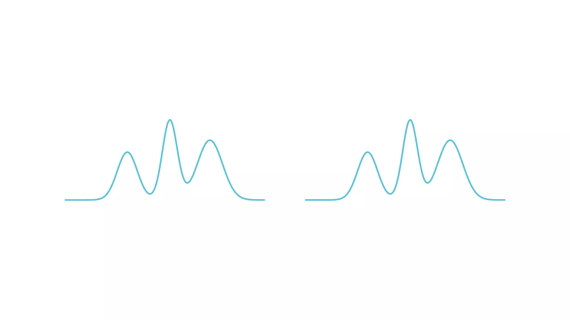
On Left, complex initial image
Red line represents guassian noise being added
On right, final Normal curve
The power of using normal (Gaussian) distributions in diffusion models comes from a fundamental property called the “stability property” of normal distributions. Here’s how it works:
When we start with any distribution (like our complex image) and add Gaussian noise to it repeatedly, the resulting distribution gradually becomes more and more Gaussian. This is due to the Central Limit Theorem, one of the most important principles in probability theory.
Think of it like mixing paint colors: If you start with any color (our original image distribution) and keep adding white paint (Gaussian noise) in small amounts, eventually your color will become consistently whitish, regardless of what color you started with. Similarly, adding Gaussian noise gradually transforms our complex image distribution into a simple Gaussian distribution.
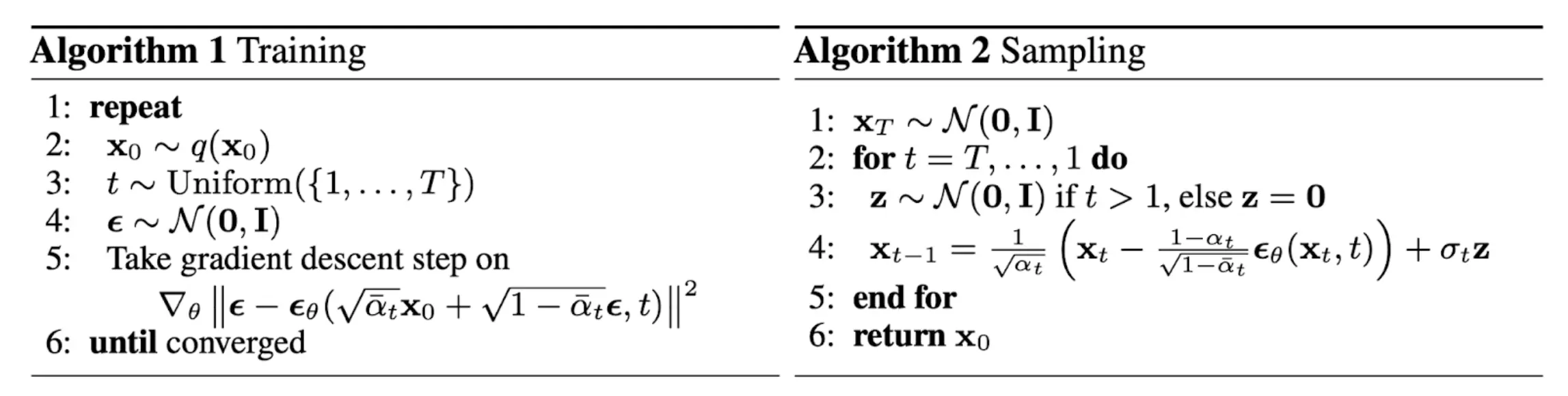
Now we understand how to add noise, how to add noise to an image at any given timestep $t$ and also why we are doing this. But how do we train a model using this? That is where the reverse diffusion process comes into the picture. As it is extremely math heavy, read about it in the maths section, here we will directly write the loss function we train over.
\[\nabla_\theta \|\epsilon - \epsilon_\theta(\sqrt{\bar{\alpha}_t}x_0 + \sqrt{1-\bar{\alpha}_t}\epsilon,t)\|^2\]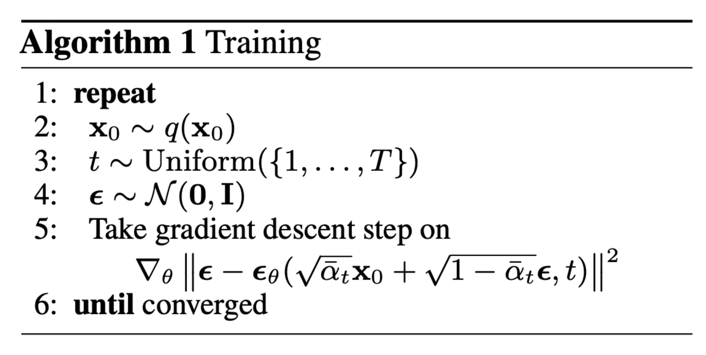
Image taken from “Denoising Diffusion Probabilistic Models”
This greatly simplifies are training, which can be written as the above image.
In summary:
- Original Artwork ($\mathbf{x}_0$): We start with a clean image from our dataset.
- Progressive Damage (t): We simulate different levels of damage by choosing a random timestep t. It’s like choosing how degraded we want our image to be.
- Adding Known Damage ($\mathbf{x}_t$): We add a specific amount of Gaussian noise to our image based on t. This is like deliberately damaging the artwork in a controlled way, where we know exactly what damage we added.
- Training the Restorer: Our neural network (like our art restorer) looks at the damaged image and tries to identify what damage was added. The loss function $|\epsilon - \epsilon_\theta(x_t,t)|_2$ measures how well the network identified the damage.
This process is efficient because:
- We can jump to any level of noise directly (thanks to the “nice property”)
- We know exactly what noise we added, so we can precisely measure how well our model predicts it
- By learning to identify the noise at any degradation level, the model implicitly learns how to restore images
This training happens in batches, where the model learns from multiple examples simultaneously, gradually improving its ability to identify and later remove noise from images.
Note: If you have played around with SD, you might know that you can switch the schedulers during inference. So is the model trained on each of these schedulers? No, The equation that we showed above just helps us train the model to predict the noise. Now we can use different schedulers (These are just mathematical equation that take noisy image & predicted noise. And return a less noisy image) to remove the noise. We have derived DDPM scheduler in the maths section
Above we discussed mainly about DDPM, but there are many kinds of schedulers. You can check few of the popular one’s here.
To know more about the differences during inference. Check this blog.
Instructions, because everyone needs guidance (Conditioning)
So far we have talked about how to generate images but have conveniently skipped over how to describe the kinds of images we want. This was another major revolution for Diffusion models, because back even when we could generate high quality images using models like GANs, it was tough to tell them what we want them to generate. Let us focus on that now.
Over the years the field of image gen has substantially improved and now we are not only limited to texts as a means of helping us generate images.
We can use image sources as guidance, a drawing of a rough idea, structure of an image etc.
As text based conditioning was the first that gained public popularity. Let’s understand more on that.
Text Encoder
The idea is relatively simple, we take texts, convert them into embeddings and send them to the U-Net layer for conditioning (whispering to Dali about what we want him to draw).
The how is more interesting if you think about it in my opinion. Throughout our discussion of diffusion models, we never talked about image description or any means to teach a model about an image.
All that a diffusion model understands is how a image looks like, without any idea about what an image is and what it contains. It’s just really good at creating images which well… look like images.
Then how can we guide it using texts about what we want it to do.
That is where CLIP comes in, first let’s understand what it does, then moving on to understand how it does it.
As I described initially, CLIP simply takes the text and converts it into embeddings.
These embeddings do not actually represent semantic meaning of text as they usually do in NLP, here they represent image structure, depth, and overall idea of an image.
These details are fed into the U-Net while the model tries to denoise the input image. With guidance from clip.
So the magic is introduced by CLIP, let us understand how CLIP was made.
CLIP (Contrastive Language–Image Pre-training)
It was originally created as a image classification tool. Given an image, describe what it.
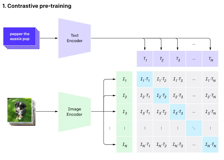
Image taken from OpenAI’s article on CLIP
Contrastive Language-Image Pre-training or CLIP pre-trains an image encoder and a text encoder which is used to predict which images are paired with which texts.
The image encoder takes images and converts them into embeddings, as you can see in the above image $I_1$ represents image 1 embeddings, $I_2$ represents image 2 embeddings and so on.
The text encoder takes captions of the images and converts them into embeddings similarily, $T_1$ for text 1 embeddings, $T_2$ for text 2 embeddings and so on.
Now as shown above, The matrix comprises of dot product of these text and image encoding. The diagonal of the matrix is maximized whereas everything else is minimized.
The diagonal of the matrix is maximized because it represents the similarity scores between correctly paired image-text pairs (e.g., $I_1 \cdot T_1$, $I_2 \cdot T_2$), while off-diagonal elements represent incorrect pairings (e.g., $I_1 \cdot T_2$). By maximizing the diagonal values through training, CLIP learns to encode semantically related images and texts into similar vector spaces, ensuring that an image’s embedding has the highest dot product with its corresponding text description’s embedding, thereby learning a shared semantic space where related visual and textual content are proximal.
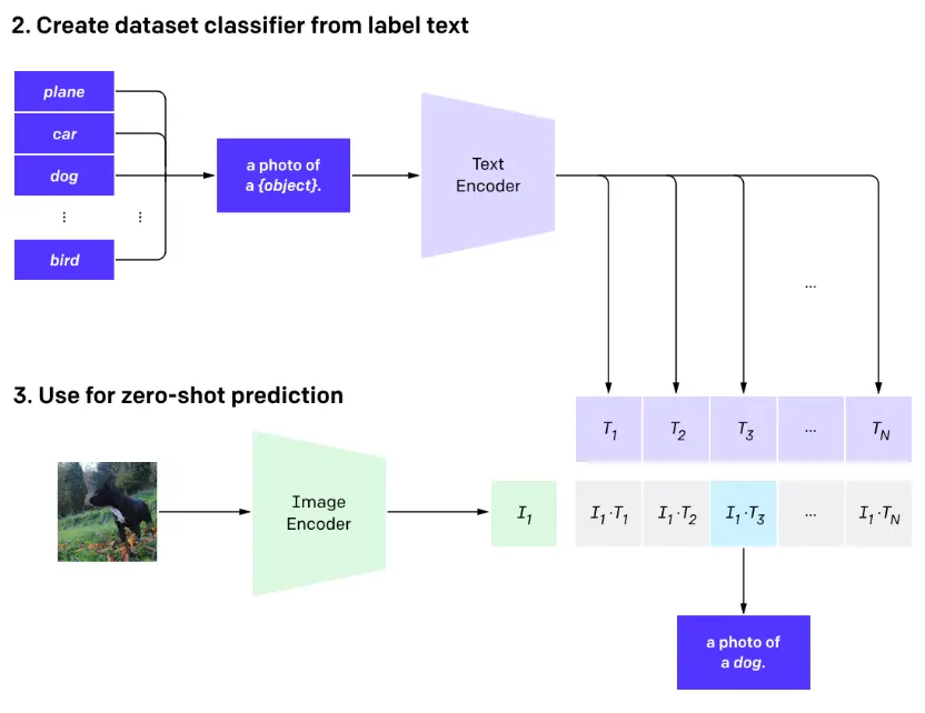
Image taken from OpenAI’s article on CLIP
Now CLIP was originally trained for zero-shot image classification. (which is a complex way of saying that “given an image, tell what it is. Without any clues”.)
As you can see from the above image, when given an image and a dataset. CLIP returns the word which has the highest dot-product (The dot-product measures the similarity) with the image encoding.
Now we primarily talked about CLIP, But there is another text encoder that is also used in practice called T5 by Google.
T5
T5 (Text-to-Text Transfer Transformer) differs from CLIP’s text encoder in several key ways:
-
Architecture & Purpose:
- CLIP’s text encoder is specifically designed for image-text alignment
- T5 is a general-purpose text model that treats every NLP task as a text-to-text problem
-
Training Approach:
- CLIP learns through contrastive learning between image-text pairs
- T5 is trained through a masked language modeling approach, where it learns to generate text by completing various text-based tasks
-
Output Use:
- In Stable Diffusion, T5 creates richer text embeddings that capture more nuanced language understanding
- These embeddings provide more detailed semantic information to guide the image generation process
The main reason Stable Diffusion uses T5 is its superior ability to understand and represent complex text descriptions, helping create more accurate and detailed image generations.
Image to Image
Image to Image is of multiple types, you can have FaceSwap, Inpainting, ControlNet etc. But all of them follow a fairly simple method. If you have understood everything so far, this part will be a ride in the park.
Control-Net
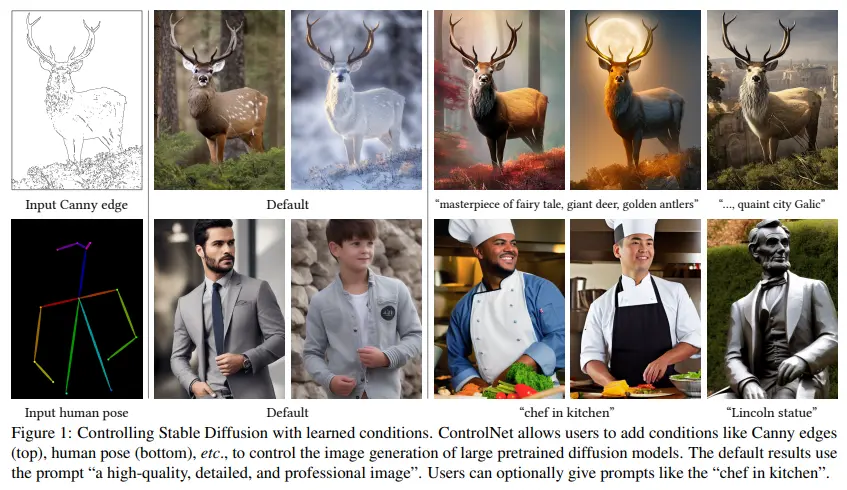
Image taken from “Adding Conditional Control to Text-to-Image Diffusion Models”
Control-Net is a popular method in the world of diffusion model, where you can take a reference image and based on that add different conditioning to achieve amazing and beautiful results. Let us understand how it works.
This part was inspired by this blog
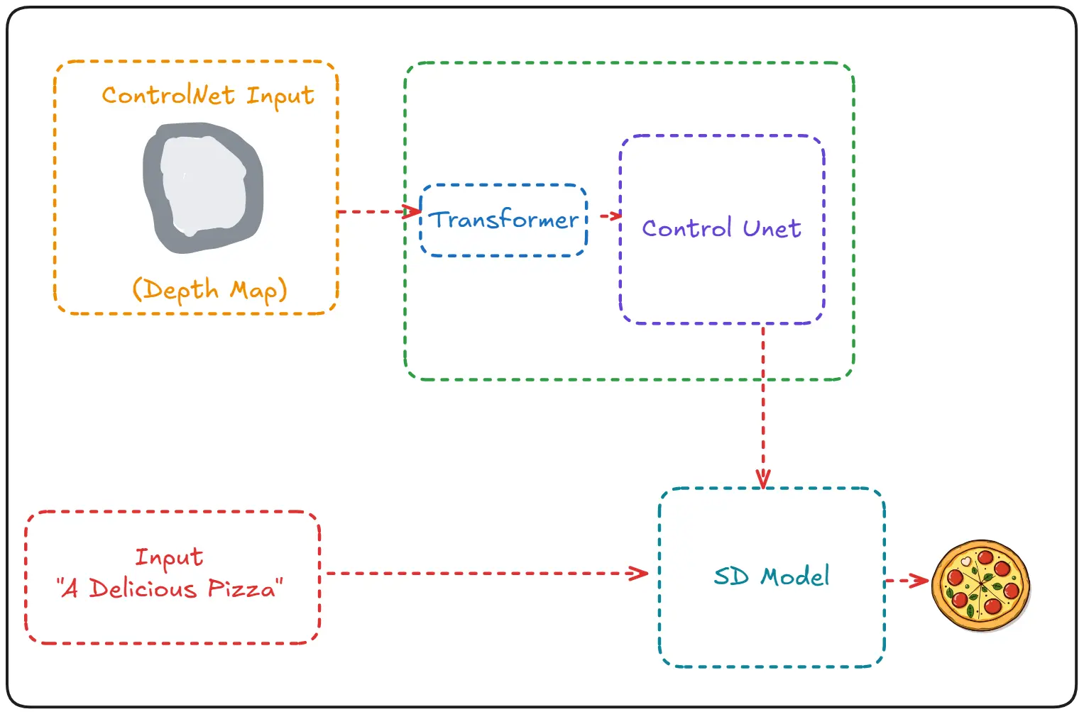
Control-Net essentially has two components ->
- The diffusion model used for generating images
- The Control-Net used for conditioning
The process itself is rather simple, we start with an image convert it into depth, canny or HUD representation. (This can be done through simple Computer Vision functions)
Then this representation is given to the Control-Net which conditions the Diffusion model during the denoising process.
Everything will make more sense when we see the internal architecture and understand how the control-net model is trained.
Note: As mentioned, a complete Control-Net model is trained for a diffusion model, so a Control-Net model trained for one model won’t work on another. For example, a control net model trained for SD1.5 cannot be used for SDXL.
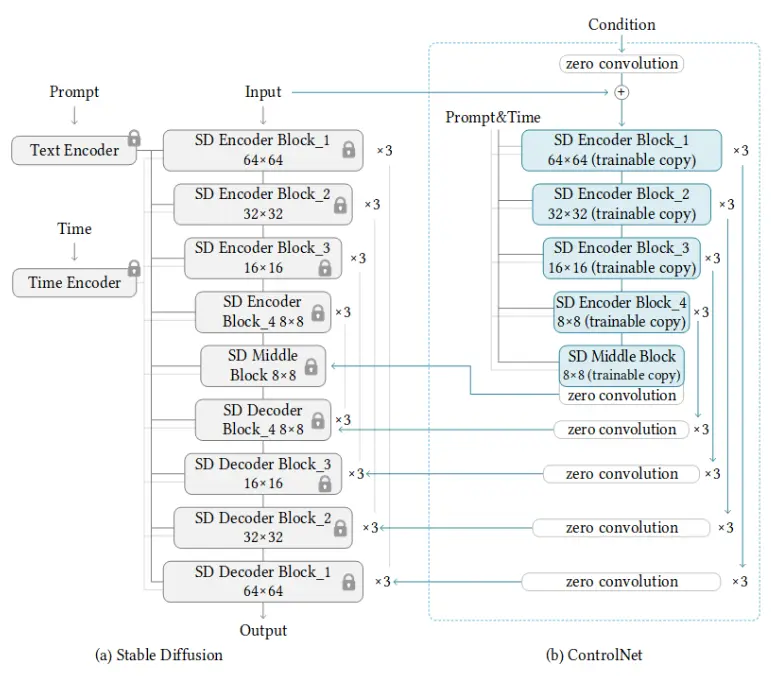
Image taken from “Adding Conditional Control to Text-to-Image Diffusion Models”
Training a Control-Net model consists of the following steps:
-
Cloning the pre-trained parameters of a Diffusion model, such as Stable Diffusion’s latent UNet(The part on the right referred to as “b”), while also maintaining the pre-trained parameters separately(The part on the left referred to as “a”).
-
“a” is kept locked, i.e not trained while training a Control-Net model to preserve the knowledge of the Diffusion model.
-
The trainable blocks of “b” are trained to learn features specific to an image.
-
The two copies (“a” and “b”) are connected through “zero convolution” layers, which are trained to bridge the locked knowledge from “a” with the new conditions being learned in “b”.
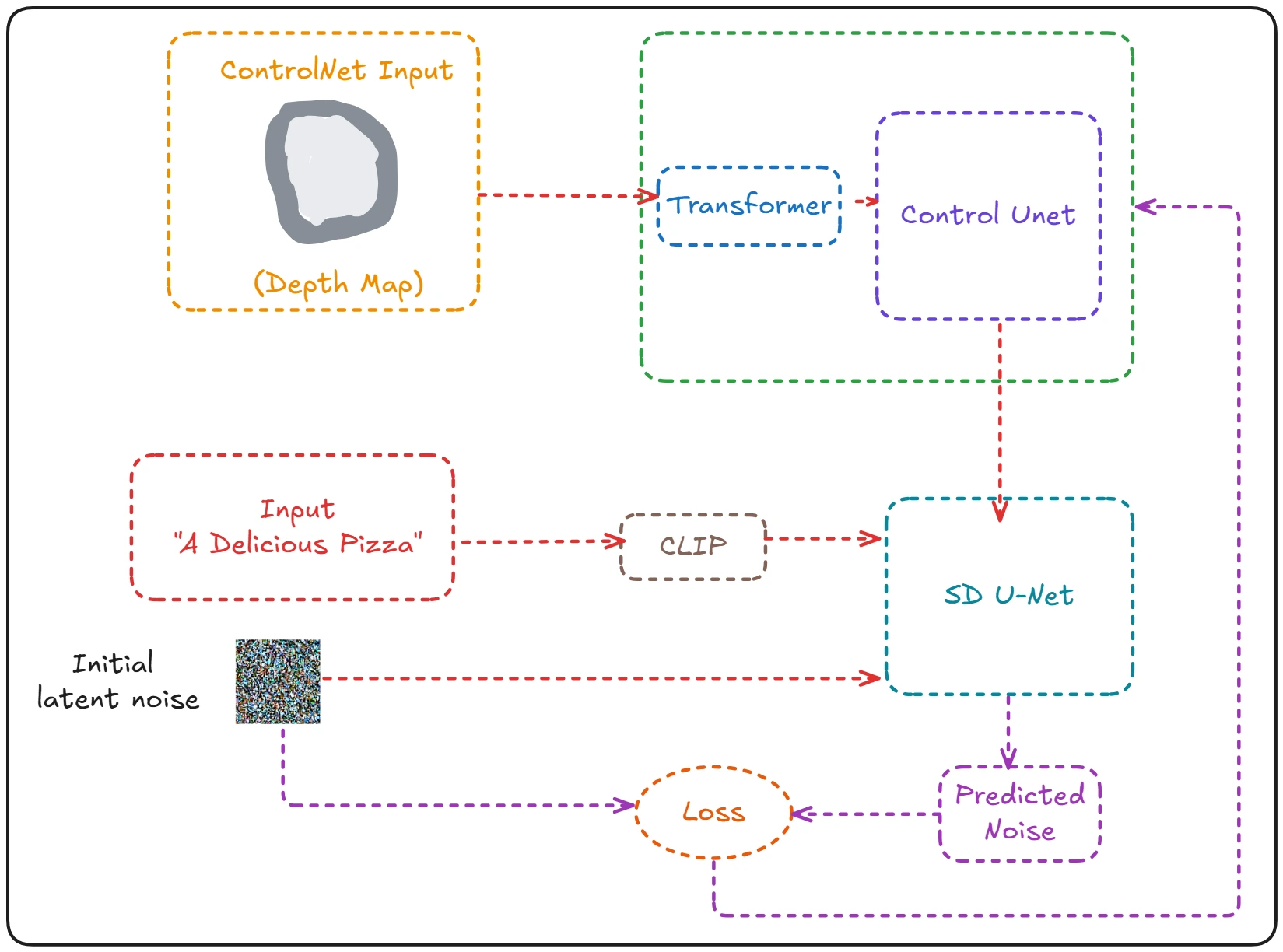
As you can see above. The SD U-Net takes in the text encoding and the noisy image. And then generates the predicted noise.
The loss calculated then is used to train the Control-Net model (inside green block)
The Control-net model consists of two parts, The transformers and the Control U-Net.
The transformer’s job is to take whatever condition we give it (depth map, edge detection etc.) and convert it into something that our U-Net can understand (latent space representation).
Think of it like this, if you are reading a book in Spanish but only know English, you will need a translator. Similarly, our U-Net only understands latent space representation, so the transformer acts as a translator converting our condition into this representation.
Let’s understand how this translation happens:
-
First Contact:
- The condition (like a depth map) goes through multiple convolution layers
- These layers are like filters that extract important features from our input
- For example, in a depth map, it might identify where objects start and end
-
Creating Understanding:
- These features are organized into a special format called a tensor
- Think of a tensor like a very organized filing cabinet where each drawer (dimension) stores specific types of information
- This tensor has information about:
- How many images we’re processing (batch size)
- The height and width of our features
- Different types of features we extracted (channels)
The ControlNet U-Net Component
ControlNet is a type of Hyper-network so let’s first understand what a Hyper-Network is:
Imagine you have a very talented artist (our base model) who is amazing at drawing pictures based on descriptions. Now, what if you want them to draw pictures based on descriptions AND reference sketches? Instead of retraining the artist (which would be time-consuming and might make them forget their original skills), we give them an assistant (hyper-network) who understands sketches and can guide the artist.
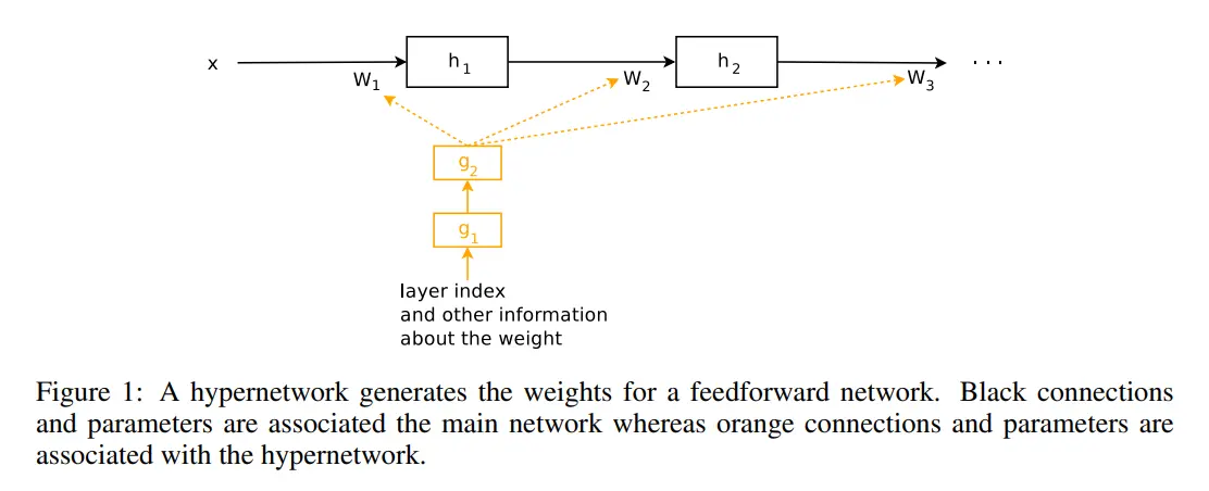
Image taken from HyperNetworks
This is exactly what ControlNet does! Instead of modifying our powerful Stable Diffusion model (the artist), it creates a smaller network (the assistant) that:
- Takes in our conditions (like depth maps, sketches)
- Processes them to extract useful information
- Guides the main model in using this information
Now, how does this guidance actually work?
Remember our U-Net from earlier? The ControlNet U-Net connects to it in a very simple way:
- It processes our condition (like a depth map)
- At each step in the U-Net, it adds its processed information to the main model’s features
- This addition subtly guides the main model without changing its learned knowledge
Think of it like this: Our artist (main model) is painting based on a description, and the assistant (ControlNet) is constantly whispering suggestions about the reference sketch, helping create an artwork that follows both the description AND the sketch.
For implementation of the original controlnet consider reading this blog, the original repo and paper
Inpainting
Let’s quickly understand inpainting - it’s like having an artist who can fill in missing or damaged parts of a photo while keeping everything else exactly the same.
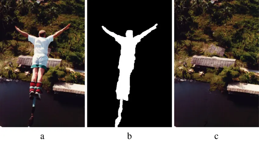
Image taken from “Image inpainting based on sparse representations with a perceptual metric”
Looking at the image above:
- In (a), we have our original image of a person jumping
- In (b), we have a mask showing which part we want to keep (in white)
- In (c), we see how we can use this information to remove the person from the scene
The magic of inpainting in diffusion models is that it only applies the denoising process to the masked areas while keeping the rest of the image unchanged. Think of it like having an artist who:
- Gets a photo with some parts erased
- Looks at the surrounding context (trees, water, buildings)
- Carefully fills in the erased parts to match perfectly with the rest
How Does It Actually Work?
Behind the scenes, inpainting uses a clever modification of our regular diffusion process. Let’s understand the technical bits:
Masked Diffusion:
   # x is our image, mask is 1 for areas to keep, 0 for areas to fill
   def add_noise_to_masked_area(x, mask, noise_level):
       noise = generate_gaussian_noise(x.shape)
       # Only add noise to masked areas (where mask = 0)
       noisy_x = x * mask + noise * (1 - mask)
       return noisy_x
We only add noise to the areas we want to fill in Original parts of the image stay untouched This preserves exact details in unmasked regions
Conditional Denoising
def denoise_step(x_t, t, mask, original_x):
    # Predict noise for the entire image
    predicted_noise = model(x_t, t)

    # Only apply denoising to masked regions
    x_t_denoised = denoise(x_t, predicted_noise)
    result = x_t_denoised * (1 - mask) + original_x * mask
    return result
The model sees both the masked and unmasked regions This helps it understand the context and maintain consistency But updates only happen in masked areas
Additional Conditioning:
The model gets extra information:
- The mask itself (where to fill)
- The surrounding context (what to match)
- Any text prompts (what to create)
This helps it generate content that fits seamlessly
Here’s how these pieces work together in practice:
def inpaint_image(original, mask, prompt):
    # Initialize with original image
    x = original.clone()

    # Step 1: Add noise only to masked region
    x_noisy = add_noise_to_masked_area(x, mask, noise_level=1.0)

    # Step 2: Gradually denoise while respecting mask
    for t in reversed(range(num_steps)):
        # Predict and denoise while maintaining original pixels
        x = denoise_step(x_noisy, t, mask, original)

        # Apply any prompt guidance
        x = apply_guidance(x, prompt, guidance_scale)

        # Ensure masked areas stay unchanged
        x = x * (1 - mask) + original * mask

    return x
This powerful technique is used for:
- Removing unwanted objects from photos
- Restoring damaged parts of old images
- Extending images beyond their original boundaries
- Creating variations of specific parts while keeping the rest intact
The best part? The same diffusion process we learned about earlier handles this naturally - it just needs to know which parts to leave alone and which parts to work on!
It is complete magic during inference. Consider reading this blog to learn more.
LoRA (Low-Rank Adaptation)
Note: Lora’s are a huge part of Image generation models and deserve an entire blog to them. Here I have tried to give a quick introduction to the idea.
Remember how earlier we talked about Dali learning the general idea of images rather than specific ones? Well, what if Dali wanted to learn a very specific style - like drawing in the style of Van Gogh, or creating anime characters? Teaching the entire model from scratch would be like making Dali relearn everything just to add one style. That would be quite inefficient!
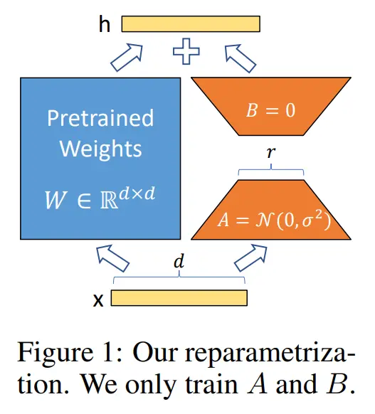
Image taken from “LoRA: Low-Rank Adaptation of Large Language Models”
This is where LoRA comes in. Instead of retraining the whole model, LoRA only modifies a tiny but crucial part - the cross-attention mechanism. Think of cross-attention as Dali’s ability to understand and connect your instructions with what he’s drawing. Let’s break this down with an example: When you say “A man with blue eyes”, two important things happen:
The model needs to understand that “blue” and “eyes” go together It needs to know where and how to draw these blue eyes in the image
The cross-attention mechanism handles these connections. It’s like Dali’s artistic intuition that knows when you say “blue eyes”, you want the eyes to be blue, not the skin or the background. LoRA works by making small adjustments to this cross-attention mechanism. Instead of teaching Dali completely new techniques, it’s like giving him a small set of notes about a specific style. These notes are much smaller (often less than 1% of the original model size!) but can significantly change how Dali draws. For example:
Want Dali to draw in anime style? Add a LoRA that tweaks how he interprets and draws faces and eyes Want more realistic portraits? A LoRA can adjust how he handles skin textures and lighting Want a specific artist’s style? LoRA can modify how he approaches colors and brush strokes
What makes LoRA especially clever is how it achieves these changes. Instead of storing full-sized modifications, it uses something called “low-rank decomposition” - think of it as finding a clever shorthand way to write down the changes. This is why LoRA files are so small compared to full models, yet can create dramatic style changes.
The Magical Wand (Variational Auto-Encoder)
This video helped me immensely while writing this part.
Unfortunately for the both of us, this part too is very maths heavy. So again I will leave the derivation for the maths section of the blog and just talk about the idea and show the equation.
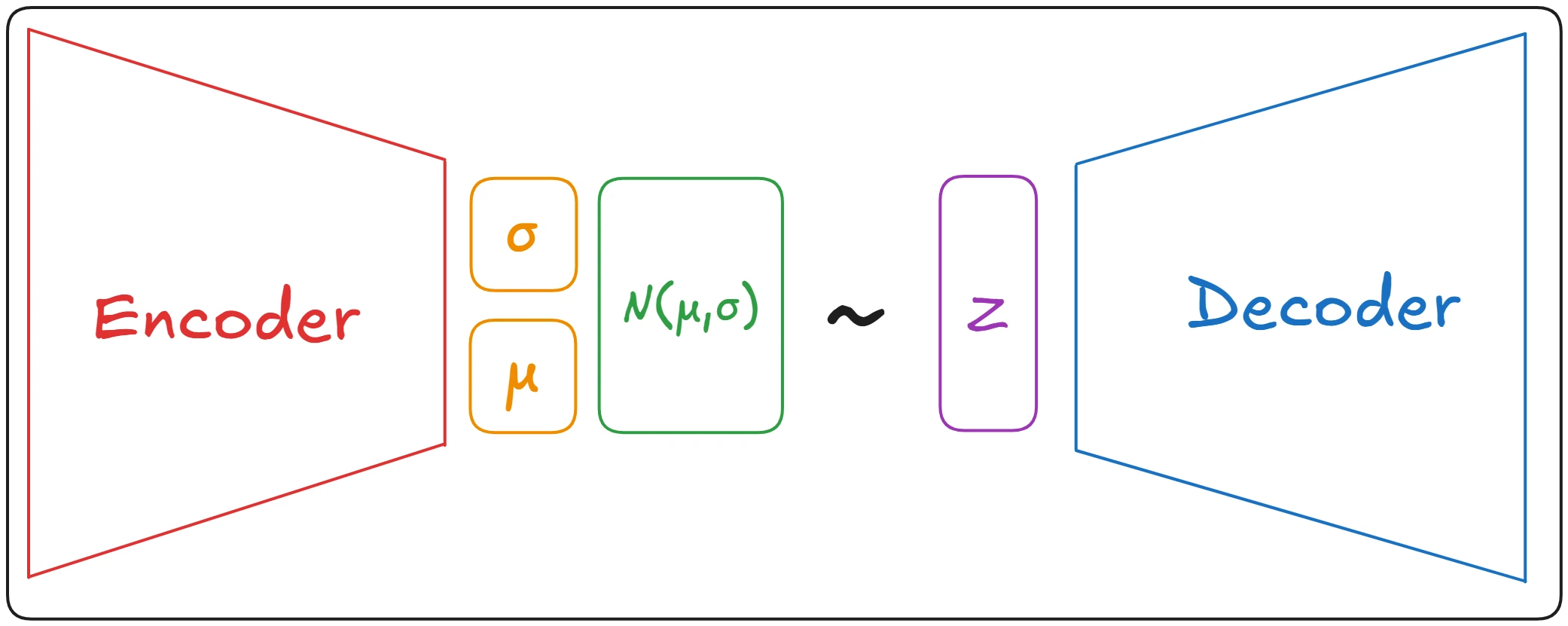 The above image is actually what happens inside of an Variational Auto-Encoder but if you are anything like me. It probably doesn’t make any sense.
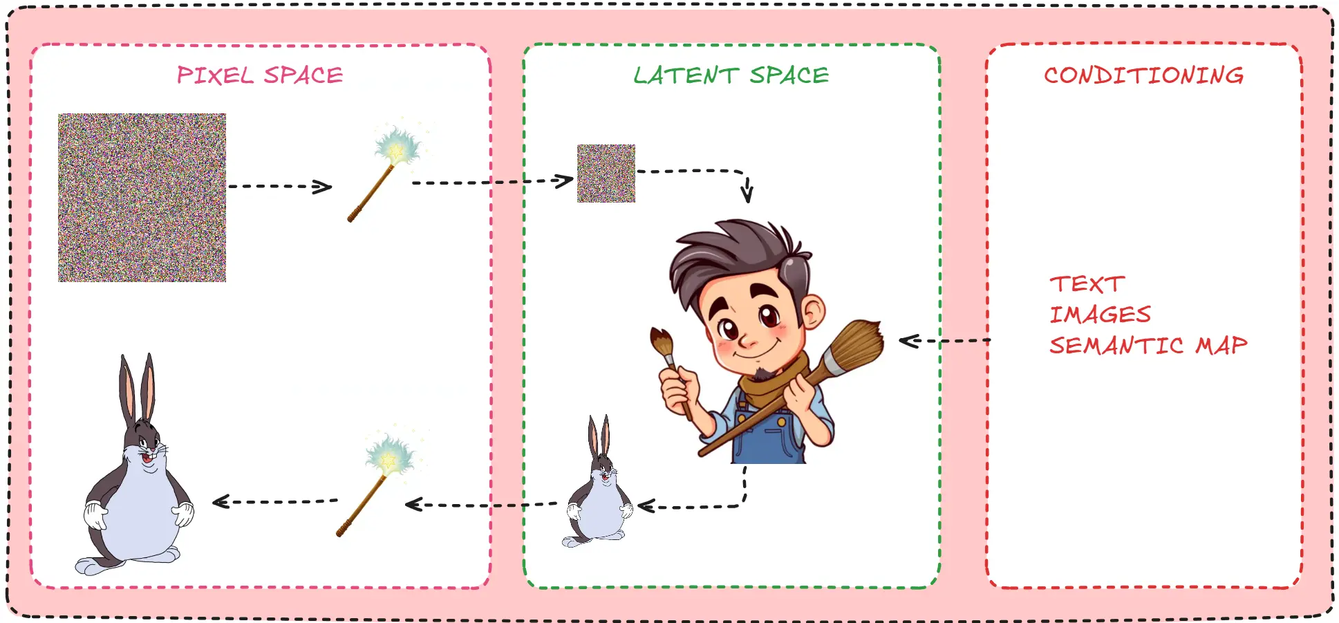
So let’s look at a simpler representation and come back to this when it makes more sense.
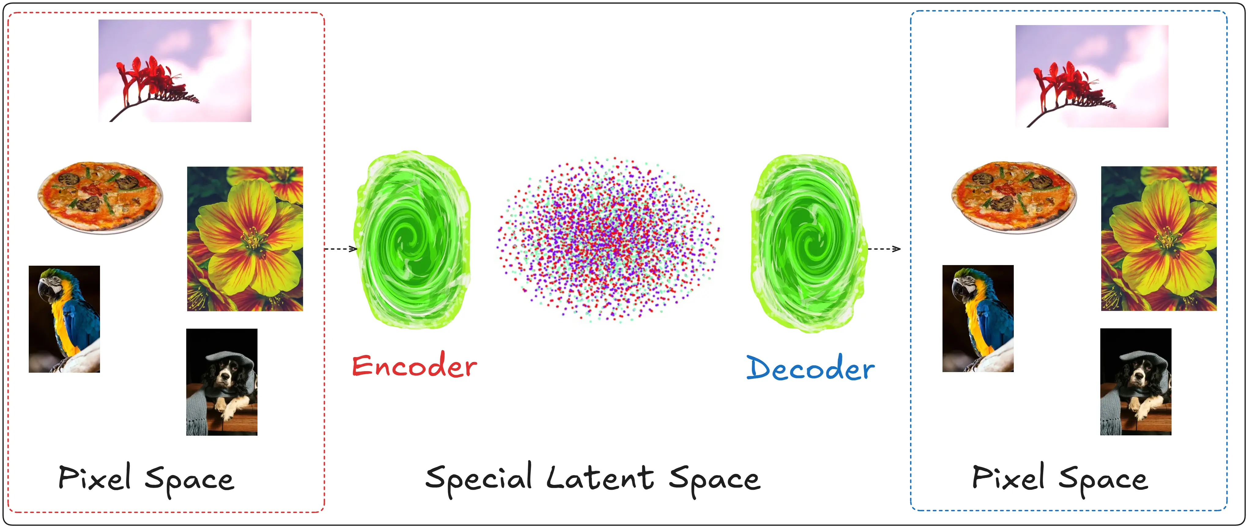
On the left side we have something called the pixel space, these are images that humans understand.
The reason it is called pixel space is pretty self-explanatory. In a computer images are made up of pixels.
The encoder takes these pixels, Yes pixels. Not the images directly. Because if we take all the pixels of an image we can form a distribution. This is how such a distribution may look like only using red, green and blue.
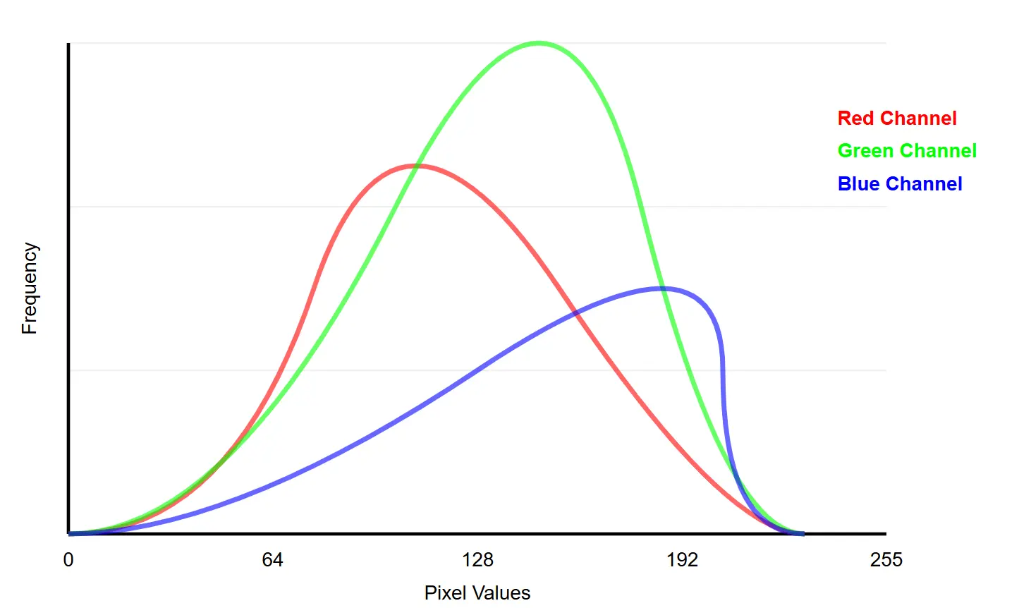
Now we take this distribution, pass it to the encoder which converts this into a latent space which has it’s own distribution.
The reason we need it is quite simple.
An HD image can be of the size 1080x1920, which is equal to 2073600 pixels. But in the latent space a representation of the same image (a representation, or in simpler terms a replica. Not the original) can be in 128X128 pixels a reduction by a factor of 126X
Then the decoder returns this representation back to pixel image so we can see a picture. Which is more or less like the original one we started with.
The reason we do this is, This makes computation substantially easier, and it also lets Dali, Or The U-Net to have to do less computation to calculate the noise.
Autoencoders (AEs) and Variational Autoencoders (VAEs) differ fundamentally in their encoding approach: Traditional autoencoders learn deterministic mappings that encode inputs directly into fixed latent vectors, while VAEs learn to encode inputs into probability distributions (typically Gaussian) in the latent space, from which latent vectors are sampled. This probabilistic nature of VAEs enables them to generate new samples and provides a more principled approach to learning continuous latent representations. To read more on this, go through the math section as well as consider reading this blog.
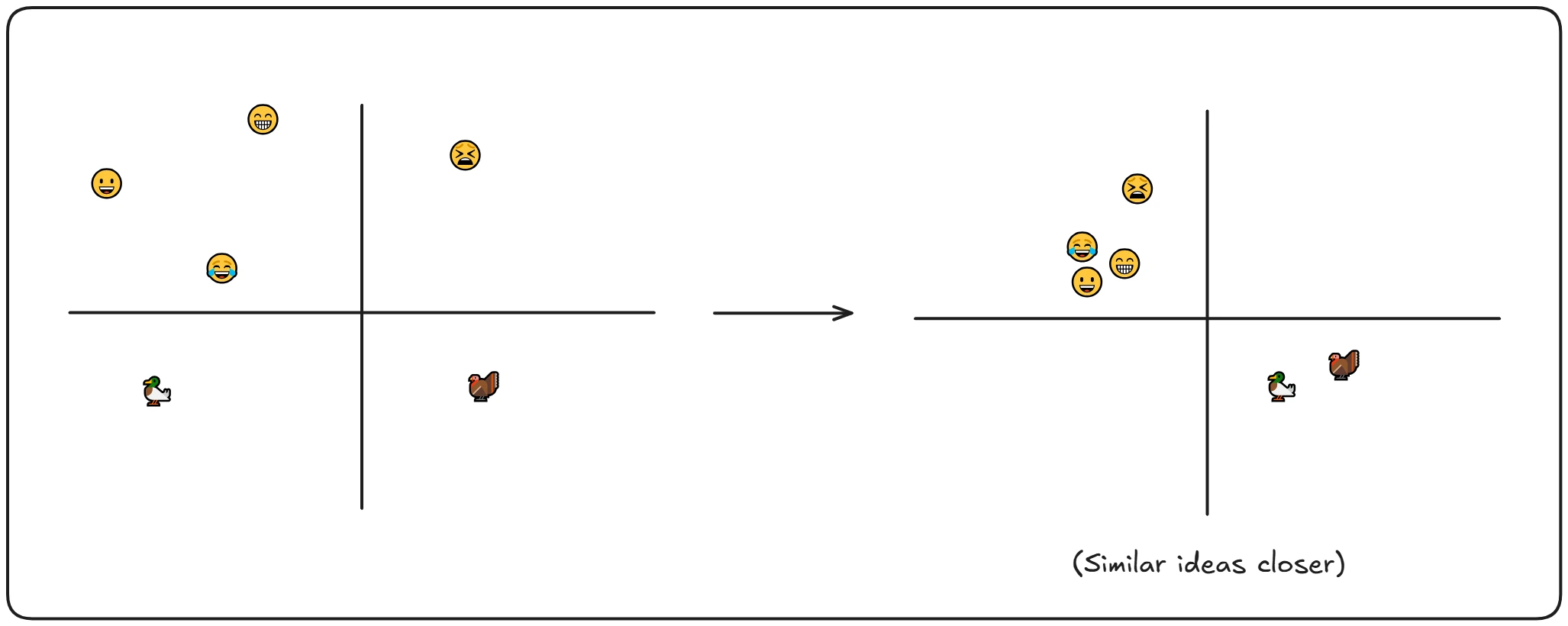
To expand on this idea, imagine a cluster of emojis—faces, animals, and other familiar icons—all grouped together in the pixel space because of their similar visual style. Now, let’s take this to the latent space. We can see that the birds are grouped together, the emojis are clustered together in another space, with similar emojis together. This demonstrates how the VAE learns to map out objects in the latent space, organizing them based on their visual or stylistic characteristics.
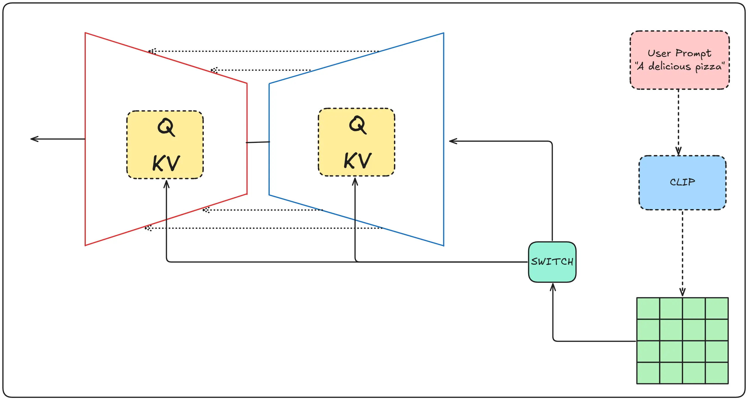
Putting it all together
A quicky Summary
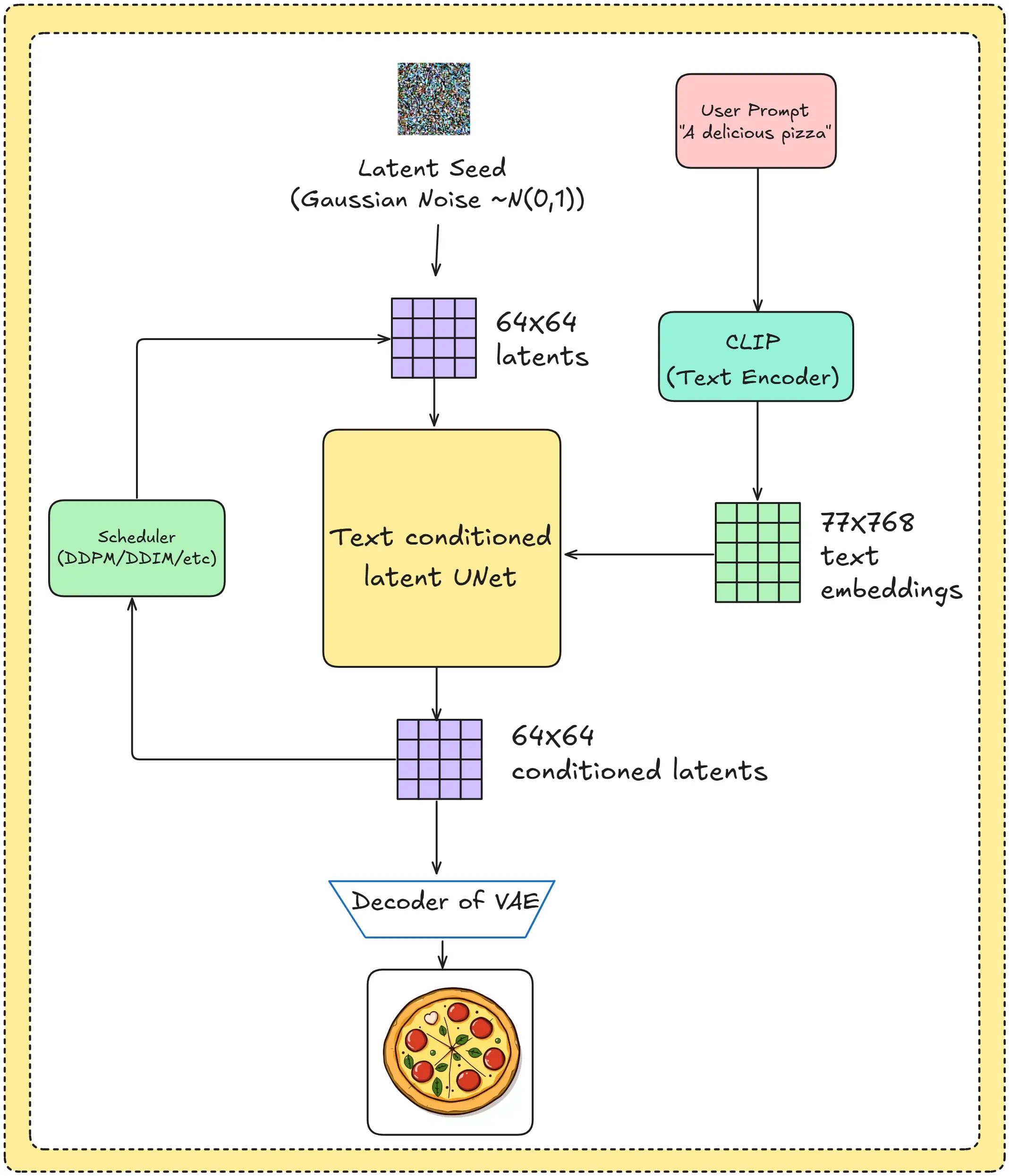
Before we move further, let’s have a quick look at everything we have understood so far.
- We begin with a prompt. (A delicious pizza)
- This prompt is converted into a text embedding using a text encoder.
- A latent noisy image is given to the U-net along with the text embeddings.
- The U-Net predicts the noise in the latents.
- The predicted noise is subtracted from the latent using the scheduler.
- After many iterations, the denoised latent is decoded using the decoder to produce our final generated image.
Note: Initially I had stated in the idea section that we start with a noisy image which is encoded. That is false, as we can simply start with a noisy latent image. Hence during inference the encoder is not required. Unless we are using it for image to image.
Also, For the scheduler we learned how we can use it to train a model. But never talked about how we can use it during inference. I.e how can we remove noise from it. More on that in the maths section.
The Dreaded Mathematics
This part was heavily influenced by the following works
As the above works were way too hard to understand. The following 3 videos really helped me out understand them
- Diffusion Models From Scratch | Score-Based Generative Models Explained | Math Explained
- Diffusion Models | Paper Explanation | Math Explained
- Denoising Diffusion Probabilistic Models | DDPM Explained
As is the nature of Understanding Stable Diffusion, it is going to be mathematics heavy. I have added an Misc & References at the bottom where you can find guides to each mathematical ideas, explained as simply as possible.
It will take too much time and distract us from the understanding of the topic at hand if I describe the mathematical ideas as well as the idea of the process in the same space.
Additionally, we will begin with the same idea that we started with when we first talked about the diffusion process. To really drive the idea home.
Maths of the Forward Diffusion process
Imagine you have a large dataset of images, we will represent this real data distribution as $q(x)$ and we take an image from it (data point/image) $x_0$. (Which is mathematically represented as $x_0 \sim q(x)$).
In the forward diffusion process we add small amounts of Gaussian noise to the image ($x_0$) in $T$ steps. Which produces a bunch of noisy images as each step which we can label as $x_1,\ldots,x_T$. These steps are controlled by a variance schedule given by $\beta_t$. The value of $\beta_t$ ranges from 0 to 1 (i.e it can take values like 0.002, 0.5,0.283 etc) for $t, \ldots, T$. (Mathematically represented as ${\beta_t \in (0,1)}_{t=1}^T$)
There are many reasons we choose Gaussian noise, but it’s mainly due to the properties of normal distribution. (about which you can read more here)
Now let us look at the big scary forward diffusion equation and understand what is going on
\[q(x_t\|x_{t-1}) = \mathcal{N}(x_t; \sqrt{1-\beta_t}x_{t-1}, \beta_t\mathbf{I}) \tag{1}\] \[q(x_{1:T}\|x_0) = \prod_{t=1}^T q(x_t\|x_{t-1}) \tag{2}\]$q(x_t|x_{t-1})$ means that given that I know $q(x_{t-1})$ what is the probability of $q(x_t)$. This is also known as bayes theorem.
To simplify it, think of it as. Given $q(x_0)$ (for value of $t$ = 1) what is the value of $q(x_1)$.
The right hand side (RHS) of equation 1 represents a normal distribution.
Now a question that I had, was how can probability and distribution be equal, well the Left Hand Side (LHS) of equation (eq) 1 represents a Probability Density Function (PDF), which is also a distribution.
For the RHS of eq 1. When we write $N(x; μ, σ²)$, we’re specifying that $x$ follows a normal distribution with mean $μ$ and variance $σ²$
This can be written as
\[p(x) = \frac{1}{\sqrt{2\pi\sigma^2}} \exp\left(-\frac{(x-\mu)^2}{2\sigma^2}\right)\]As $t$ becomes larger. And eventually when $T \to \infty$ (This means as $T$ approaches infinity, or just a really large number). The initial data sample $x_0$ loses its features and turns into an Isotropic Gaussian Distribution.
Whilst eq 2 looks complex, it simply means. Given the original image $x_0$ all the values of $x_t$ from $t=1$ to $t=T$ are equal to, multiplication of the PDF from $t=1$ to $t=T$
Let’s talk about an interesting property - we can actually sample $x_t$ at any arbitrary timestep (This is the “nice property”). This means we don’t need to go through the diffusion process step by step to get to a specific noise level.
First, let’s understand something fundamental about normal distributions. Any normal distribution can be represented in the following form:
\[X = \mu + \sigma \epsilon\]where $\epsilon \sim \mathcal{N}(0,1)$ (This means $\epsilon$ is sampled from a normal distribution with mean 0 and variance 1)
Taking our equation from before:
\[q(x_t|x_{t-1}) = \mathcal{N}(x_t; \sqrt{1-\beta_t}x_{t-1}, \beta_t\mathbf{I})\]We can rewrite this using the above form as:
\[x_t = \sqrt{1-\beta_t}x_{t-1} + \sqrt{\beta_t}\epsilon_{t-1}\]To make our equations simpler, let’s define $\alpha_t = 1-\beta_t$. This gives us:
\[x_t = \sqrt{\alpha_t}x_{t-1} + \sqrt{1-\alpha_t}\epsilon_{t-1}\]Now, we can substitute the expression for $x_{t-1}$ in terms of $x_{t-2}$ (in the above equation just replace $t$ with $t-1$):
\[x_t = \sqrt{\alpha_t}(\sqrt{\alpha_{t-1}}x_{t-2} + \sqrt{1-\alpha_{t-1}}\epsilon_{t-2}) + \sqrt{1-\alpha_t}\epsilon_{t-1}\]A key property of normal distributions is that when we add two normal distributions, their means and variances can be combined. Using this property and some algebraic manipulation, we get:
\[x_t = \sqrt{\alpha_t\alpha_{t-1}}x_{t-2} + \sqrt{1-\alpha_t\alpha_{t-1}}\bar{\epsilon}_{t-2}\]If we continue this process all the way back to our original image \(x_0\), and define \(\bar{\alpha}_t\) as the product of all \(\alpha\)s from 1 to t (\(\bar{\alpha}_t = \prod_{i=1}^t \alpha_i\)), we arrive at:
\[x_t = \sqrt{\bar{\alpha}_t}x_0 + \sqrt{1-\bar{\alpha}_t}\epsilon\]This final equation is quite powerful. As tt allows us to directly sample $x_t$ at any timestep $t$ using just:
- The original image $x_0$
- The cumulative product of alphas up to time $t$ ($\bar{\alpha}_t$)
- A sample from a standard normal distribution ($\epsilon$)
This makes our implementation much more efficient as we can directly jump to any noise level without calculating all the intermediate steps.
Maths of Reverse diffusion process
Note: If you have made it this far, you should be immensely proud of yourself. It is not easy to make sense of all the mathematics that you have made sense of so far. Be proud because ML mathematics will only ever get sightlier more complex than this. This is the upper limit, which you have reached with your tenacity.
Reverse diffusion process
Now what we want to do is take a noisy image $x_t$ and get the original image $x_0$ from it. And to do that we need to do a reverse diffusion process.
Essentially we want to sample from $q(x_{t-1}|x_t)$, Which is quite tough as there can be millions of noisy images for actual images. To combat this we create an approximation (why do they work and how do they work in a minute) $p_\theta$ to approximate these conditional probabilities in order to run the reverse diffusion process.
Which can be represented as
\[p_\theta(x_{t-1}|x_t) = \mathcal{N}(x_{t-1}; \mu_\theta(x_t,t), \Sigma_\theta(x_t,t))\] \[p_\theta(x_{0:T}) = p(x_T)\prod_{t=1}^T p_\theta(x_{t-1}|x_t)\](Notice how the above two equation are very similar to the equations we started out with for the forward diffusion process)
Unfortunately it is tough to even sample from this approximate model because it is the same as our previous model, so we modify it by adding the original image $x_0$ to it as such.
\[q(x_{t-1}|x_t,x_0) = \mathcal{N}(x_{t-1}; {\color{Blue}{}\tilde{\mu}(x_t,x_0)}, {\color{red}{}\tilde{\beta}_t\mathbf{I}})\]Now this is tractable (I.e computationally possible), let us first understand why it is tractable. Later moving on to using this to generate a loss function.
When we only condition on $x_t$ (the noisy image) with the equation \(p_\theta(x_{t-1}\|x_t)\), our model faces a significant challenge. Imagine trying to guess what a slightly less noisy version of a noisy image should look like, without any reference to the original image. There are countless possibilities! This makes the problem intractable because:
- The model needs to consider all possible original images that could have resulted in $x_t$
- For each possibility, it needs to calculate the probability of that being the correct original image
- It then needs to integrate over all these possibilities to make its prediction
This is computationally infeasible and lacks a closed-form solution.
When we modify our formulation to include $x_0$, creating \(q(x_{t-1}\|x_t,x_0)\), several wonderful mathematical properties emerge:
-
Complete Information:
- We now know both the starting point ($x_0$) and current point $x_t$
- This means we can calculate exactly how much noise was added during the forward process
- The randomness becomes deterministic when we have this information
-
Gaussian Properties:
- Our forward process $q(x_t|x_0)$ is Gaussian
- Thanks to the properties of Gaussian distributions, $q(x_{t-1}|x_t,x_0)$ is also Gaussian
- This gives us closed-form solutions for the mean and variance
Here’s a concrete analogy: Imagine trying to guess the middle point of a line:
- If you only know one endpoint $x_t$, there are infinite possible middle points
- If you know both endpoints ($x_t$ and $x_0$), you can calculate the middle point exactly
Why This Works in Practice
During training, this approach is perfectly feasible because:
Training Phase:
- We have access to x₀ (original images)
- We can calculate the exact posterior $q(x_{t-1}\|x_t,x_0)$
- Our model learns to approximate this posterior distribution
Inference Phase:
- We only need $p_\theta(x_{t-1}\|x_t)$
- The model has learned the patterns of noise removal
- We can generate new images without needing $x_0$
Mathematical Insight
The key mathematical insight is that by conditioning on $x_0$, we transform an intractable marginalization problem into a tractable direct computation. Our posterior becomes:
\[q(x_{t-1}|x_t,x_0) = \mathcal{N}(x_{t-1}; \tilde{\mu}(x_t,x_0), \tilde{\beta}_t\mathbf{I})\]Where both μ̃ and β̃_t have closed-form solutions that we can compute efficiently.
This formulation gives us the best of both worlds:
- Tractable mathematics during training
- Practical applicability during inference
By leveraging this insight, diffusion models can effectively learn the reverse process while keeping the mathematics manageable and computationally feasible.
Now using the equation and Bayes’ rule, we have:
\[\begin{aligned} q(x_{t-1}|x_t,x_0) &= \frac{q(x_t|x_{t-1},x_0)q(x_{t-1}|x_0)}{q(x_t|x_0)} & \text{[Bayes' Rule: } P(A|B) = \frac{P(B|A)P(A)}{P(B)} \text{]} \end{aligned}\]Since $q(x)$ represents a normal distribution, we can expand using the general form of a normal distribution:
\[\mathcal{N}(x|\mu,\sigma^2) = \frac{1}{\sqrt{2\pi\sigma^2}}\exp(-\frac{(x-\mu)^2}{2\sigma^2})\]Therefore:
\[\begin{aligned} q(\mathbf{x}_{t-1} \vert \mathbf{x}_t, \mathbf{x}_0) &= q(\mathbf{x}_t \vert \mathbf{x}_{t-1}, \mathbf{x}_0) \frac{ q(\mathbf{x}_{t-1} \vert \mathbf{x}_0) }{ q(\mathbf{x}_t \vert \mathbf{x}_0) } \\ &\propto \exp \Big(-\frac{1}{2} \big(\frac{(\mathbf{x}_t - \sqrt{\alpha_t} \mathbf{x}_{t-1})^2}{\beta_t} + \frac{(\mathbf{x}_{t-1} - \sqrt{\bar{\alpha}_{t-1}} \mathbf{x}_0)^2}{1-\bar{\alpha}_{t-1}} - \frac{(\mathbf{x}_t - \sqrt{\bar{\alpha}_t} \mathbf{x}_0)^2}{1-\bar{\alpha}_t} \big) \Big) \\ &= \exp \Big(-\frac{1}{2} \big(\frac{\mathbf{x}_t^2 - 2\sqrt{\alpha_t} \mathbf{x}_t \color{blue}{\mathbf{x}_{t-1}} \color{black}{+ \alpha_t} \color{red}{\mathbf{x}_{t-1}^2} }{\beta_t} + \frac{ \color{red}{\mathbf{x}_{t-1}^2} \color{black}{- 2 \sqrt{\bar{\alpha}_{t-1}} \mathbf{x}_0} \color{blue}{\mathbf{x}_{t-1}} \color{black}{+ \bar{\alpha}_{t-1} \mathbf{x}_0^2} }{1-\bar{\alpha}_{t-1}} - \frac{(\mathbf{x}_t - \sqrt{\bar{\alpha}_t} \mathbf{x}_0)^2}{1-\bar{\alpha}_t} \big) \Big) \\ &= \exp\Big( -\frac{1}{2} \big( \color{red}{(\frac{\alpha_t}{\beta_t} + \frac{1}{1 - \bar{\alpha}_{t-1}})} \mathbf{x}_{t-1}^2 - \color{blue}{(\frac{2\sqrt{\alpha_t}}{\beta_t} \mathbf{x}_t + \frac{2\sqrt{\bar{\alpha}_{t-1}}}{1 - \bar{\alpha}_{t-1}} \mathbf{x}_0)} \mathbf{x}_{t-1} \color{black}{ + C(\mathbf{x}_t, \mathbf{x}_0) \big) \Big)} \end{aligned}\]Note: Notice the proportionality sign (\(\propto\)) in the 1st step of the derivation. This shows that we are omitting the constants (\(\frac{1}{\sqrt{2\pi\sigma^2}}\)) for now. Also in the next step we have simply used \((A + B)^2 = A^2 + 2AB + B^2\)
where $C(x_t,x_0)$ is some function not involving $x_{t-1}$, hence details can be omitted.
If we have a look again at our equation of normal distribution:
\[\mathcal{N}(x|\mu,\sigma^2) = \frac{1}{\sqrt{2\pi\sigma^2}}\exp(-\frac{(x-\mu)^2}{2\sigma^2})\]Expanding the squared term in the exponential:
\[\exp(-\frac{1}{2\sigma^2}(x^2 - 2\mu x + \mu^2))\]The coefficient of $x^2$ is $\frac{1}{2\sigma^2}$, and the coefficient of $x$ is $-\frac{\mu}{\sigma^2}$. All other terms not involving $x$ can be collected into the normalization constant.
Therefore, comparing this with our previous equation:
\[\color{red}{(\frac{\alpha_t}{\beta_t}+\frac{1}{1-\bar{\alpha}_{t-1}})} = \frac{1}{2\sigma^2}\]and
\[\color{blue}{(\frac{2\sqrt{\alpha_t}}{\beta_t}x_t+\frac{2\sqrt{\bar{\alpha}_{t-1}}}{1-\bar{\alpha}_{t-1}}x_0)} = \frac{2\mu}{\sigma^2}\]Following the above logic, the mean (\(\tilde{\mu}_t(x_t,x_0)\)) and variance (\(\tilde{\beta}_t\)) can be parameterized as follows (recall that \(\alpha_t=1-\beta_t\) and \(\bar{\alpha}_t=\prod_{i=1}^t \alpha_i\)):
\[\begin{aligned} \tilde{\beta}_t &= 1/(\frac{\alpha_t}{\beta_t}+\frac{1}{1-\bar{\alpha}_{t-1}}) \\ &= 1/(\frac{\alpha_t-\bar{\alpha}_t+\beta_t}{\beta_t(1-\bar{\alpha}_{t-1})}) \\ &= \color{yellow}{}\frac{1-\bar{\alpha}_{t-1}}{1-\bar{\alpha}_t}\cdot\beta_t \end{aligned}\] \[\begin{aligned} \tilde{\mu}_t(x_t,x_0) &= (\frac{\alpha_t}{\beta_t}x_t+\frac{\bar{\alpha}_{t-1}}{1-\bar{\alpha}_{t-1}}x_0)/(\frac{\alpha_t}{\beta_t}+\frac{1}{1-\bar{\alpha}_{t-1}}) \\ &= (\frac{\alpha_t}{\beta_t}x_t+\frac{\bar{\alpha}_{t-1}}{1-\bar{\alpha}_{t-1}}x_0)\color{yellow}\frac{1-\bar{\alpha}_{t-1}}{1-\bar{\alpha}_t}\cdot\beta_t \\ &= \frac{\alpha_t(1-\bar{\alpha}_{t-1})}{1-\bar{\alpha}_t}x_t+\frac{\bar{\alpha}_{t-1}\beta_t}{1-\bar{\alpha}_t}x_0 \end{aligned}\]Let’s break down this derivation step by step:
-
We start with a complex fraction that has terms involving both \(x_t\) and \(x_0\). This is our initial mean equation.
-
To simplify this complex fraction, we use a common mathematical technique: multiply both numerator and denominator by the same term (which is equivalent to multiplying by 1). In this case, we multiply by \(\frac{1-\bar{\alpha}_{t-1}}{1-\bar{\alpha}_t}\cdot\beta_t\) (shown in yellow).
-
After distributing terms and simplifying:
- The \(\frac{\alpha_t}{\beta_t}\) term combines with \(\beta_t\) to give us just \(\alpha_t\)
- The fraction \(\frac{\bar{\alpha}_{t-1}}{1-\bar{\alpha}_{t-1}}\) simplifies when multiplied by \((1-\bar{\alpha}_{t-1})\)
- All terms get divided by \((1-\bar{\alpha}_t)\) due to our multiplication
This gives us our final simplified form where the mean is expressed as two clean terms, one involving \(x_t\) and one involving \(x_0\).
Thanks to the nice property, we can represent \(x_0=\frac{1}{\sqrt{\bar{\alpha}_t}}(x_t-\sqrt{1-\bar{\alpha}_t}\epsilon_t)\) and replacing \(x_0\) in the above equation:
\[\begin{aligned} \tilde{\mu}_t &= \frac{\alpha_t(1-\bar{\alpha}_{t-1})}{1-\bar{\alpha}_t}x_t+\frac{\bar{\alpha}_{t-1}\beta_t}{1-\bar{\alpha}_t}\cdot\frac{1}{\sqrt{\bar{\alpha}_t}}(x_t-\sqrt{1-\bar{\alpha}_t}\epsilon_t) \\ &= \frac{\alpha_t(1-\bar{\alpha}_{t-1})}{1-\bar{\alpha}_t}x_t+\frac{\bar{\alpha}_{t-1}\beta_t}{1-\bar{\alpha}_t}\cdot\frac{x_t}{\sqrt{\bar{\alpha}_t}}-\frac{\bar{\alpha}_{t-1}\beta_t}{1-\bar{\alpha}_t}\cdot\frac{\sqrt{1-\bar{\alpha}_t}}{\sqrt{\bar{\alpha}_t}}\epsilon_t \end{aligned}\]Using the property that \(\bar{\alpha}_t = \bar{\alpha}_{t-1}\alpha_t\) and \(\beta_t = 1-\alpha_t\), we can simplify to get:
\[\tilde{\mu}_t = \frac{1}{\alpha_t}(x_{t-1}-\frac{\alpha_t}{\sqrt{1-\bar{\alpha}_t}}\epsilon_t)\]This is great, we now have the mean in terms of \(x_{t-1}\) and it does not depend on the original image \(x_0\). The key mathematical properties used in this derivation are:
- \(\bar{\alpha}_t = \bar{\alpha}_{t-1}\alpha_t\) (product of alphas)
- \(\beta_t = 1-\alpha_t\) (relationship between beta and alpha)
- The reparameterization of \(x_0\) in terms of \(x_t\) and \(\epsilon_t\)
Note: Constants like 2,1/2,K etc have been omitted in many places as they do not hold much significance to the final equation
Now we have the mean, which can help us denoise the image. But we still need a training objective, using which the model gradually learns the approximation function.
Training Loss ($L_t$)
Our original objective was to create an approcimate conditional probability distribution using which we could train a neural network to reverse the diffusion process.
\[p_\theta(\mathbf{x}_{t-1}\|\mathbf{x}_t) = \mathcal{N}(\mathbf{x}_{t-1}; \boldsymbol{\mu}_\theta(\mathbf{x}_t, t), \boldsymbol{\Sigma}_\theta(\mathbf{x}_t, t)).\]We wish to train $\boldsymbol{\mu}_\theta$ to predict $\tilde{\boldsymbol{\mu}}_t$. Because $\mathbf{x}_t$ is available as input at training time.
But through all our toil, we can reparameterize the Gaussian noise term to make it predict $\boldsymbol{\epsilon}_t$ from the input $\mathbf{x}_t$ at timestep $t$:
\[\boldsymbol{\mu}_\theta(\mathbf{x}_t, t) = \frac{1}{\sqrt{\alpha_t}}(\mathbf{x}_t - \frac{1-\alpha_t}{\sqrt{1-\bar{\alpha}_t}}\boldsymbol{\epsilon}_\theta(\mathbf{x}_t, t))\]Thus \(\mathbf{x}_{t-1} = \mathcal{N}(\mathbf{x}_{t-1}; \frac{1}{\sqrt{\alpha_t}}(\mathbf{x}_t - \frac{1-\alpha_t}{\sqrt{1-\bar{\alpha}_t}}\boldsymbol{\epsilon}_\theta(\mathbf{x}_t, t)), \boldsymbol{\Sigma}_\theta(\mathbf{x}_t, t))\)
The loss term $L_t$ is parameterized to minimize the difference from $\tilde{\boldsymbol{\mu}}$:
\[L_t = \mathbb{E}_{\mathbf{x}_0,\boldsymbol{\epsilon}}\left[\frac{1}{2\|\boldsymbol{\Sigma}_\theta(\mathbf{x}_t, t)\|_2^2}\|\tilde{\boldsymbol{\mu}}_t(\mathbf{x}_t, \mathbf{x}_0) - \boldsymbol{\mu}_\theta(\mathbf{x}_t, t)\|^2\right]\]This scary looking equation is simply the Mean Squared Error for an estimator. (MSE is a popular loss function in ML)
Also given as,
\[\begin{align*} \text{MSE}(\hat{\theta}) &= \mathbb{E}_{\theta}\left[(\hat{\theta} - \theta)^2\right] \\ &= \mathbb{E}_{\mathbf{x}_0,\boldsymbol{\epsilon}}\left[\frac{1}{2\|\boldsymbol{\Sigma}_\theta\|_2^2}\|\frac{1}{\sqrt{\alpha_t}}(\mathbf{x}_t - \frac{1-\alpha_t}{\sqrt{1-\bar{\alpha}_t}}\boldsymbol{\epsilon}_t) - \frac{1}{\sqrt{\alpha_t}}(\mathbf{x}_t - \frac{1-\alpha_t}{\sqrt{1-\bar{\alpha}_t}}\boldsymbol{\epsilon}_\theta(\mathbf{x}_t, t))\|^2\right] \\ &= \mathbb{E}_{\mathbf{x}_0,\boldsymbol{\epsilon}}\left[\frac{(1-\alpha_t)^2}{2\alpha_t(1-\bar{\alpha}_t)\|\boldsymbol{\Sigma}_\theta\|_2^2}\|\boldsymbol{\epsilon}_t - \boldsymbol{\epsilon}_\theta(\mathbf{x}_t, t)\|^2\right] \\ &= \mathbb{E}_{\mathbf{x}_0,\boldsymbol{\epsilon}}\left[\frac{(1-\alpha_t)^2}{2\alpha_t(1-\bar{\alpha}_t)\|\boldsymbol{\Sigma}_\theta\|_2^2}\|\boldsymbol{\epsilon}_t - \boldsymbol{\epsilon}_\theta(\sqrt{\bar{\alpha}_t}\mathbf{x}_0 + \sqrt{1-\bar{\alpha}_t}\boldsymbol{\epsilon}_t, t)\|^2\right] \end{align*}\]Simplification
Ho et al. in “Denoising Diffusion Probabilistic Models” found that training the diffusion model works better with a simplified objective that ignores the weighting term:
\[\begin{align*} L_t^{\text{simple}} &= \mathbb{E}_{t\sim[1,T],\mathbf{x}_0,\boldsymbol{\epsilon}_t}[\|\boldsymbol{\epsilon}_t - \boldsymbol{\epsilon}_\theta(\mathbf{x}_t,t)\|^2] \\ &= \mathbb{E}_{t\sim[1,T],\mathbf{x}_0,\boldsymbol{\epsilon}_t}[\|\boldsymbol{\epsilon}_t - \boldsymbol{\epsilon}_\theta(\sqrt{\bar{\alpha}_t}\mathbf{x}_0 + \sqrt{1-\bar{\alpha}_t}\boldsymbol{\epsilon}_t,t)\|^2] \end{align*}\]The final simple objective is:
$L^{\text{simple}} = L_t^{\text{simple}} + C$
where $C$ is a constant not depending on $\theta$.
Hence the equations simply become
Congratulations, you have a complete understanding of how we came to these equations now. Do not take from granted to how these equations were reached. We have skipped over a lot of the groundbreaking mathematical ideas which led to the creation of the above equation. Read more here.
Score Based Modeling
“ Langevin dynamics is a concept from physics, developed for statistically modeling molecular systems. Combined with stochastic gradient descent, stochastic gradient Langevin dynamics (Welling & Teh 2011) can produce samples from a probability density $p(x)$ using only the gradients $\nabla_x \log p(x)$ in a Markov chain of updates:
\(x_t = x_{t-1} + \frac{\delta}{2}\nabla_x \log p(x_{t-1}) + \sqrt{\delta}\epsilon_t, \text{ where } \epsilon_t \sim \mathcal{N}(0,\mathbf{I})\)
where $\delta$ is the step size. When $T \to \infty, \delta \to 0$, $x_T$ equals to the true probability density $p(x)$.
Compared to standard SGD, stochastic gradient Langevin dynamics injects Gaussian noise into the parameter updates to avoid collapses into local minima.
“
From Lil’s Blog
Score based modeling, was a revolutionary idea that set the stones for further progress in diffusion model.
It is a fascinating bridge between physics and machine learning!
First, let’s understand what Langevin dynamics is trying to do. Imagine you’re trying to find the lowest point in a hilly landscape while blindfolded. If you only walk downhill (like regular gradient descent), you might get stuck in a small valley that isn’t actually the lowest point. Langevin dynamics solves this by occasionally taking random steps - like sometimes walking uphill - which helps you explore more of the landscape. The key equation is:
\[x_t = x_{t-1} + \frac{\delta}{2}\nabla_x \log p(x_{t-1}) + \sqrt{\delta}\epsilon_t\]Let’s break this down piece by piece:
$x_t$ and $x_{t-1}$ represent our position at the current and previous steps.
$\nabla_x \log p(x_{t-1})$ is the gradient term - it tells us which direction to move to increase the probability
δ is our step size - how far we move in each step
ϵt is our random noise term, sampled from a normal distribution
The equation combines two behaviors:
A “deterministic” part: $\frac{\delta}{2}\nabla_x \log p(x_{t-1})$ which moves us toward higher probability regions
A “random” part: $\sqrt{\delta}\epsilon_t$ which adds noise to help us explore
What makes this special is that when we run this process for a long time (\(T\rightarrow\infty\)) and with very small steps (\(\delta\rightarrow0\)), we’re guaranteed to sample from the true probability distribution \(p(x)\). This is similar to how diffusion models gradually denoise images - they’re following a similar kind of path, but in reverse!
The connection to standard gradient descent is interesting - regular SGD would only have the gradient term, but Langevin dynamics adds that noise term \(\epsilon_t\). This noise prevents us from getting stuck in bad local minima, just like how shaking a jar of marbles helps them settle into a better arrangement.
This is already immensely helpful, Because if we recall our previous discussion. Our biggest issue had been how do we create an approximate of our distribution because it is computationally expensive.
Now, here’s the key insight of Langevin dynamics: When we take the gradient of log probability (\(\nabla\log p(x)\)), we get something called the “score function”. This score function has a special property - it points in the direction where the probability increases most rapidly.
Let’s see why through calculus:
\[\nabla\log p(x) = \nabla(\log p(x)) = \frac{1}{p(x)}\nabla p(x)\]This division by \(p(x)\) acts as an automatic scaling factor. When \(p(x)\) is small, it makes the gradient larger, and when \(p(x)\) is large, it makes the gradient smaller. This natural scaling helps our sampling process explore the probability space more efficiently.
What is \(p(x)\) though and why are we taking that. Traditionally in SGD do we take, $\frac{\partial(\text{error})}{\partial(\text{weight})}$
In traditional SGD for neural networks, we’re trying to minimize an error function (or loss function), so we use \(\frac{\partial(\text{error})}{\partial(\text{weight})}\). We’re trying to find the weights that make our predictions as accurate as possible.
But in Langevin dynamics, we’re doing something fundamentally different. Here, \(p(x)\) represents a probability distribution that we want to sample from. Think of it this way:
Imagine you have a dataset of faces, and you want to generate new faces that look real. The probability \(p(x)\) would represent how likely it is that a particular image \(x\) is a real face. Areas of high \(p(x)\) would correspond to images that look like real faces, while areas of low \(p(x)\) would be images that don’t look like faces at all.
So when we take \(\nabla\log p(x)\), we’re asking: “In which direction should I move to make this image look more like a real face?”
This is why Langevin dynamics is particularly relevant to diffusion models. Remember how diffusion models start with noise and gradually transform it into an image? The \(\nabla\log p(x)\) term tells us how to modify our noisy image at each step to make it look more like real data.
To learn more about Score Based Modeling, consider reading this blog by Yang Song
The Score Function: Bridging Diffusion and Guidance
Remember how we started with our forward diffusion process? We had:
\[q(x_t|x_0) = \mathcal{N}(x_t; \sqrt{\bar{\alpha}_t}x_0, (1-\bar{\alpha}_t)\mathbf{I})\]This equation tells us the probability distribution of our noisy image $x_t$ given the original image $x_0$. Now, here’s where things get interesting. The score function we mentioned in the score-based modeling section is defined as:
\[\text{score}(x) = \nabla_x \log p(x)\]When we apply this to our forward diffusion process $q(x_t|x_0)$, we can derive our key equation. Let’s do this step by step:
-
First, let’s write out the log probability for a Gaussian distribution:
\[\log q(x_t|x_0) = -\frac{(x_t - \sqrt{\bar{\alpha}_t}x_0)^2}{2(1-\bar{\alpha}_t)} + C\]where $C$ is a normalization constant we can ignore for the gradient.
-
Taking the gradient with respect to $x_t$:
\[\nabla_{x_t}\log q(x_t|x_0) = -\frac{x_t - \sqrt{\bar{\alpha}_t}x_0}{1-\bar{\alpha}_t}\] -
Remember our reparameterization trick from earlier? We can express $x_0$ in terms of $x_t$ and $\epsilon$:
\[x_0 = \frac{1}{\sqrt{\bar{\alpha}_t}}(x_t - \sqrt{1-\bar{\alpha}_t}\epsilon_t)\] -
Substituting this in:
\[\nabla_{x_t}\log q(x_t|x_0) = -\frac{x_t - \sqrt{\bar{\alpha}_t}(\frac{1}{\sqrt{\bar{\alpha}_t}}(x_t - \sqrt{1-\bar{\alpha}_t}\epsilon_t))}{1-\bar{\alpha}_t}\] -
After simplifying (and some algebra that we’ll skip for sanity), we get:
\[\nabla_{x_t}\log q(x_t) = -\frac{1}{1-\bar{\alpha}_t}\epsilon_t\] -
In practice, we use our model’s prediction $\epsilon_\theta(x_t,t)$ instead of the true noise $\epsilon_t$, giving us our final equation:
\[\nabla_{x_t}\log q(x_t) = -\frac{1}{1-\bar{\alpha}_t}\epsilon_\theta(x_t,t)\]
This equation is powerful because it connects three key concepts:
- The forward diffusion process (through $\bar{\alpha}_t$)
- The noise prediction model (through $\epsilon_\theta$)
- The score function (through $\nabla_{x_t}\log q$)
Understanding this connection is crucial because it shows us why the noise prediction approach works - it’s actually learning to estimate the score function scaled by a constant factor! This is why we can use it in our guidance equations, as it tells us how to modify our noisy image to make it more like what we want.
Note: The score function interpretation is particularly elegant because it shows that our diffusion model isn’t just randomly removing noise - it’s learning the underlying structure of the probability distribution of real images. When we do guidance, we’re essentially tweaking this learned structure to better match our prompts.
Mathematics of Guidance in Diffusion Models
Let’s understand how we can mathematically guide our diffusion process to better follow our prompts. There are two main approaches: Classifier Guidance and Classifier-Free Guidance (CFG).
Classifier Guidance
First, recall that our diffusion process tries to predict and remove noise. The base noise prediction is:
\[\nabla_{x_t}\log q(x_t) = -\frac{1}{1-\bar{\alpha}_t}\epsilon_\theta(x_t,t)\]When we want to incorporate class or prompt information $y$, we can write the score function for the joint distribution $q(x_t,y)$ as:
\[\nabla_{x_t}\log q(x_t,y) = \nabla_{x_t}\log q(x_t) + \nabla_{x_t}\log q(y|x_t)\]This looks complex, but the idea is simple - we’re combining:
- How the image should evolve naturally ($\nabla_{x_t}\log q(x_t)$)
- How it should change to better match our prompt ($\nabla_{x_t}\log q(y|x_t)$)
We can approximate this using a classifier $f_\phi(y|x_t)$:
\[\nabla_{x_t}\log q(x_t,y) \approx -\frac{1}{1-\bar{\alpha}_t}\epsilon_\theta(x_t,t) + \nabla_{x_t}\log f_\phi(y|x_t)\]This gives us our classifier-guided noise predictor:
\[\bar{\epsilon}_\theta(x_t,t) = \epsilon_\theta(x_t,t) - (1-\bar{\alpha}_t)\nabla_{x_t}\log f_\phi(y|x_t)\]And to control how strongly we follow the classifier’s guidance, we add a weight $w$:
\[\bar{\epsilon}_\theta(x_t,t) = \epsilon_\theta(x_t,t) - (1-\bar{\alpha}_t)w\nabla_{x_t}\log f_\phi(y|x_t)\]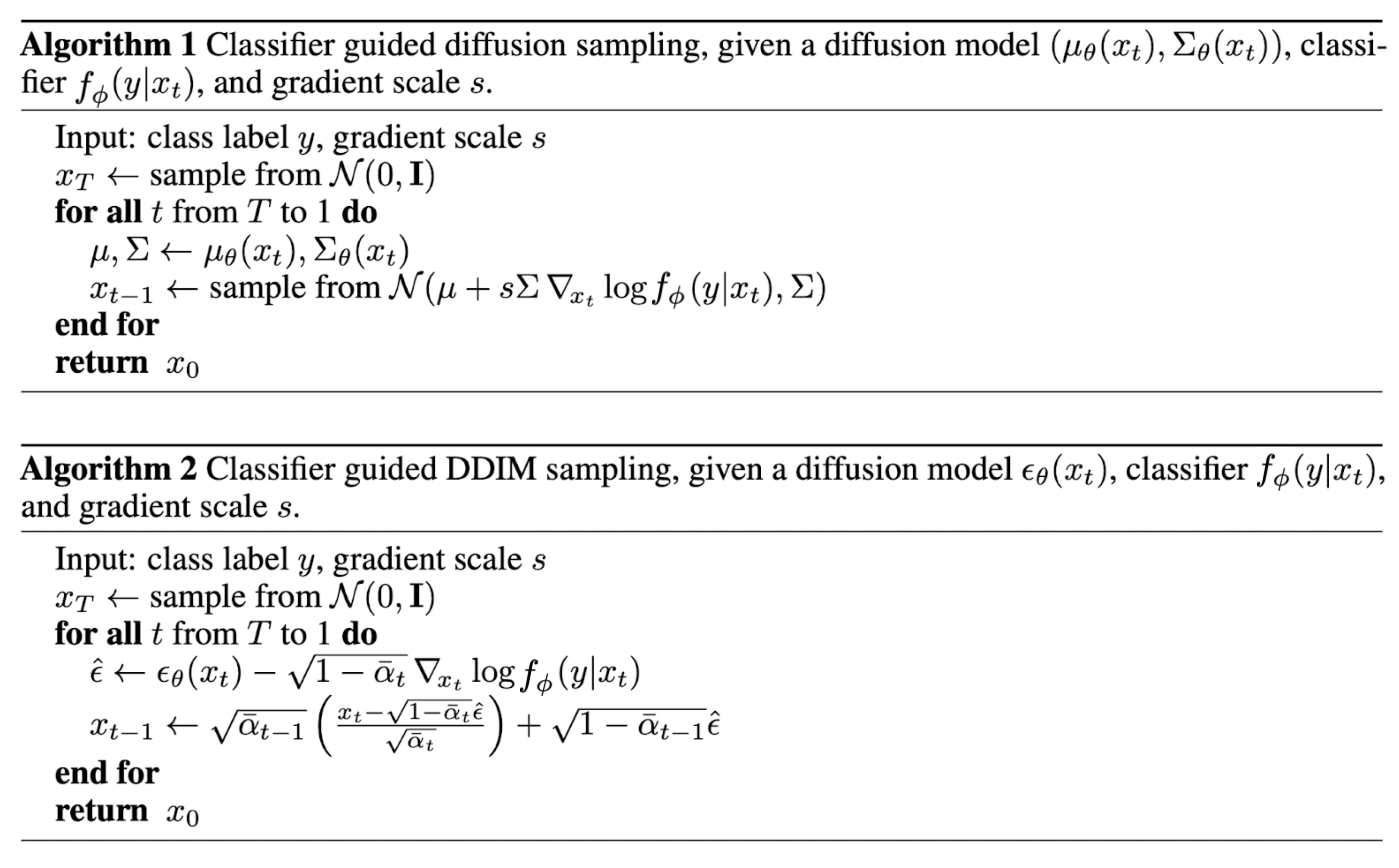
Image taken from “Diffusion Models Beat GANs on Image Synthesis”
Classifier-Free Guidance
CFG takes a different approach. Instead of training a separate classifier, we use the same model to predict noise both with and without conditioning.
Let’s say we have:
- $\epsilon_\theta(x_t,t)$: Unconditional noise prediction
- $\epsilon_\theta(x_t,t,y)$: Conditional noise prediction (using prompt)
The gradient of an implicit classifier can be written as:
\[\nabla_{x_t}\log p(y|x_t) = \nabla_{x_t}\log p(x_t|y) - \nabla_{x_t}\log p(x_t)\] \[= -\frac{1}{1-\bar{\alpha}_t}(\epsilon_\theta(x_t,t,y) - \epsilon_\theta(x_t,t))\]When we plug this into our guidance formula, we get:
\[\bar{\epsilon}_\theta(x_t,t,y) = \epsilon_\theta(x_t,t,y) + w(\epsilon_\theta(x_t,t,y) - \epsilon_\theta(x_t,t))\]Which simplifies to:
\[\bar{\epsilon}_\theta(x_t,t,y) = (w+1)\epsilon_\theta(x_t,t,y) - w\epsilon_\theta(x_t,t)\]This final equation is what most modern diffusion models use. The weight $w$ (often called the CFG scale) controls how much we want our generation to follow the prompt:
- $w = 0$: Pure unconditional generation
- $w = 1$: Normal conditional generation
- $w > 1$: Increased adherence to the prompt
The beauty of CFG is its simplicity - we don’t need a separate classifier, just the difference between conditional and unconditional predictions from our main model.
Note:There is still a lot of things that we can discuss like LDMs, Distillation etc. But now you have the essential idea for majority of how SD maths work. So you can tackle it on your own, you can check more about it here.
Maths of VAE
This part of blog takes inspiration from Lilian’s blog on VAE and Jaan’s Blog on the topic.
To understand the mathematics behind VAE lets begin by setting some conventions first:
- $x$ represents a real input data point (an image)
- $z$ represents the latent space variables
- $p(z)$: The prior - what we think z should look like before seeing any data
- $p(x|z)$: The likelihood - how to generate data from the latent representation
- $p(z|x)$: The posterior - given data, what’s its latent representation?
The central idea is we have a latent space $z$ and when we sample a data point $x^*_i$ from it, we want it to be as close as possible to the original datapoint $x_i$
This is represented mathematically as $p(z|x)$ (Think right to left: given x, we want to get z)
From Bayes’ formula we can write:
\[p(z|x) = \frac{p(x|z)p(z)}{p(x)}\]We can calculate $p(x)$ as:
\[p(x) = \int p(x|z)p(z)dz\](This equation comes from The Law of Total Probability)
Unfortunately, this integral is computationally very expensive as we need to evaluate it over all possible configurations of latent variables.
Hence instead of calculating $p(z|x)$ directly, we calculate an approximation $q_{\lambda}(z|x)$, parameterized by $\lambda$. For example, if $q$ were Gaussian, $\lambda$ would represent the mean and variance of the latent variables for each datapoint: $\lambda_{x_i} = (\mu_{x_i}, \sigma^2_{x_i})$.
Now how do we know how close this approximation is to our original data distribution? That is where KL Divergence comes in.
What is KLD? Kullback-Leibler Divergence (KLD) measures how different two probability distributions are from each other. Think of it as measuring the “distance” between distributions, but it’s not a true distance because it’s asymmetric ($KL(P|Q) \neq KL(Q|P)$). In our case, we use it to measure how far our approximation $q_{\lambda}(z|x)$ is from the true posterior $p(z|x)$. The smaller the KLD, the better our approximation.
KLD deserves an entire blog on its own. Due to time & length constraints, I am recommending the following two blogs, which will help you get the whole idea ASAP. Blog 1 & Blog 2.
Using KLD we can write:
\[KL(q_{\lambda}(z|x)||p(z|x)) = E_q[\log q_{\lambda}(z|x)] - E_q[\log p(x,z)] + \log p(x)\]We want to find a value of $\lambda$ that minimizes the difference between these two distributions. Which we can write as:
\[q^*_{\lambda}(z|x) = \arg\min_{\lambda} KL(q_{\lambda}(z|x)||p(z|x))\]Sadly, even this is intractable (hard to compute) as we again have our $p(z|x)$ term in it.
So we introduce ELBO (Evidence Lower BOund), which provides us with a tractable way to optimize our model. ELBO represents the lower bound on the evidence (log probability) of our observed data. It is written as:
\[ELBO(\lambda) = E_q[\log p(x,z)] - E_q[\log q_{\lambda}(z|x)]\]Notice how we can combine this with the equation of KLD we wrote earlier and get the following formula:
\[\log p(x) = ELBO(\lambda) + KL(q_{\lambda}(z|x)||p(z|x))\]What is ELBO? ELBO is a clever mathematical trick that gives us a way to maximize $p(x)$ indirectly. Instead of computing the intractable $p(x)$ directly, we compute a lower bound that’s easier to calculate. Think of it like measuring the height of a building - instead of climbing to measure the exact height (intractable), we measure its shadow and use trigonometry (tractable). The beauty of ELBO is that when we maximize it, we’re also maximizing $p(x)$, since ELBO is always less than or equal to $\log p(x)$.
By Jensen’s inequality, the KLD is always greater than or equal to zero. Hence if we minimize KLD we will maximize ELBO. This makes our lives easier as we can indeed calculate the ELBO.
We can decompose the ELBO for a single data point as following:
\[ELBO_i(\lambda) = E_{q_{\lambda}(z|x_i)}[\log p(x_i|z)] - KL(q_{\lambda}(z|x_i)||p(z))\]We can see that this is equivalent to our previous definition of ELBO through the following derivation:
Starting with our original ELBO:
\[ELBO(\lambda) = E_q[\log p(x,z)] - E_q[\log q_{\lambda}(z|x)]\]We can expand $\log p(x,z)$ using the chain rule of probability:
\[\log p(x,z) = \log p(x|z) + \log p(z)\]Substituting this back:
\[ELBO(\lambda) = E_q[\log p(x|z) + \log p(z)] - E_q[\log q_{\lambda}(z|x)]\]Using the linearity of expectation:
\[ELBO(\lambda) = E_q[\log p(x|z)] + E_q[\log p(z)] - E_q[\log q_{\lambda}(z|x)]\]Rearranging terms:
\[ELBO(\lambda) = E_q[\log p(x|z)] - (E_q[\log q_{\lambda}(z|x)] - E_q[\log p(z)])\]The term in parentheses is exactly the KL divergence between $q_{\lambda}(z|x)$ and $p(z)$, giving us:
\[ELBO(\lambda) = E_q[\log p(x\|z)] - KL(q_{\lambda}(z|x)||p(z))\]Which is the same as our single-point ELBO formula.
The Reparameterization Trick
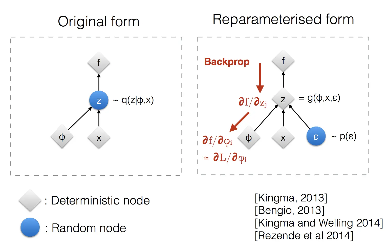
Image taken from “From Autoencoder to Beta-VAE by Lillian Weng”
There’s a critical problem we haven’t addressed yet. Remember our ELBO formula:
\[ELBO_i(\lambda,\phi) = E_{q_{\lambda}(z|x_i)}[\log p_{\phi}(x_i|z)] - KL(q_{\lambda}(z|x_i)||p(z))\]To optimize this, we need to calculate gradients through the entire process. However, sampling from $q_{\lambda}(z|x_i)$ is a random operation, and we can’t backpropagate through random sampling!
The Problem
- Our encoder outputs parameters for a probability distribution (usually mean $\mu$ and variance $\sigma^2$ for a Gaussian)
- We sample $z$ from this distribution
- We can’t compute gradients through this random sampling step
The Solution: Reparameterization Trick
Instead of directly sampling $z$, we:
- Sample a random noise $\epsilon$ from a standard normal distribution $\mathcal{N}(0,1)$
- Transform it using our distribution parameters:
where $\odot$ represents element-wise multiplication.
This is equivalent to sampling from $\mathcal{N}(\mu, \sigma^2)$, but now the randomness is separated from the network parameters!
Why This Works
- The random sampling ($\epsilon$) is now independent of the network parameters
- $\mu$ and $\sigma$ are direct outputs of our encoder network
- We can backpropagate through this transformation
- During backpropagation, $\epsilon$ is treated as a constant
In practice, our VAE now looks like this:
- Encoder outputs $\mu$ and $\sigma$
- Sample $\epsilon \sim \mathcal{N}(0,1)$
- Compute $z = \mu + \sigma \odot \epsilon$
- Feed $z$ into decoder
- Calculate loss and backpropagate
This trick is what makes VAEs trainable in practice!
Connecting to Neural Networks
Now that we understand the mathematical foundation, let’s see how this translates to actual neural networks.
The key insight is that we can implement our probability distributions using neural networks:
-
The Encoder Network (Inference Network)
- Takes input data $x$ and outputs parameters $\lambda$
- Implements our approximate posterior $q_{\lambda}(z|x)$
- Parameters $\lambda$ are the weights and biases of this network
-
The Decoder Network (Generative Network)
- Takes latent variables $z$ and reconstructs the data
- Implements our likelihood $p_{\phi}(x|z)$
- Parameters $\phi$ are the weights and biases of this network
With these networks, we can rewrite our ELBO formula to include the network parameters:
\[ELBO_i(\lambda,\phi) = E_{q_{\lambda}(z|x_i)}[\log p_{\phi}(x_i|z)] - KL(q_{\lambda}(z|x_i)||p(z))\]This formula serves as our loss function (technically its negative):
\[Loss_i(\lambda,\phi) = -ELBO_i(\lambda,\phi)\]Let’s break down what each term means in practice:
-
First Term: $E_{q_{\lambda}(z|x_i)}[\log p_{\phi}(x_i|z)]$
- This is our reconstruction loss
- How well can we reconstruct the input after encoding and decoding?
- Think of it as “How close is the output to the input?”
-
Second Term: $KL(q_{\lambda}(z|x_i)||p(z))$
- This is our regularization term
- Keeps our latent space well-behaved
- Makes sure our encoded representations don’t deviate too far from our prior
We optimize this loss function using stochastic gradient descent, which:
- Updates encoder parameters ($\lambda$) to better approximate the posterior
- Updates decoder parameters ($\phi$) to better reconstruct the input
Note: This is called variational EM (Expectation Maximization) because we’re maximizing the expected log-likelihood of our data with respect to both sets of parameters.
And that’s it! We’ve connected the dots between probability theory and neural networks. The VAE is essentially:
- An encoder that compresses data into a well-behaved latent space
- A decoder that reconstructs data from this latent space
- A loss function that ensures both good reconstruction and well-structured latent representations
The code
Let’s Gradually make this section more complex, starting with the quickest way to start generating images to the more complex methods
This website is an amazing starting point to understand what each line of code does. Consider checking it out, it helped me significantly while writing this section.
The following section takes significant help from the following two sources
Diffusers by Huggingface
This section takes inspiration from the blog Stable Diffusion with 🧨 Diffusers by HuggingFace
from diffusers import StableDiffusionPipeline

pipe = StableDiffusionPipeline.from_pretrained("CompVis/stable-diffusion-v1-4")
pipe.to("cuda")

prompt = "a photograph of an astronaut riding a horse"

image = pipe(prompt).images[0]

# you can save the image with
# image.save(f"astronaut_rides_horse.png")
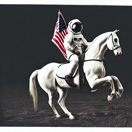
As surprsing as it may seem, you only need the above 5 lines to start generating images using SD.
This is nice, but what is the point of everything we have learned if we stick to just abstraction layers. Lets move forward
If you wish to modify the different components without actually coding them out, that is also possible using diffusers. Consider reading this blog to understand how to do that.
VAE
import torch
import torch.nn as nn
import torch.nn.functional as F

class Encoder(nn.Module):
    def __init__(self, in_channels=3, latent_dim=4):
        super().__init__()
        # Convolutional layers for feature extraction
        # Each conv layer reduces spatial dimensions by 2 and increases channels
        self.conv1 = nn.Conv2d(in_channels, 32, kernel_size=3, stride=2, padding=1)
        self.conv2 = nn.Conv2d(32, 64, kernel_size=3, stride=2, padding=1)
        self.conv3 = nn.Conv2d(64, 128, kernel_size=3, stride=2, padding=1)
        self.conv4 = nn.Conv2d(128, 256, kernel_size=3, stride=2, padding=1)

        # Batch normalization layers for training stability
        self.bn1 = nn.BatchNorm2d(32)
        self.bn2 = nn.BatchNorm2d(64)
        self.bn3 = nn.BatchNorm2d(128)
        self.bn4 = nn.BatchNorm2d(256)

        # Linear layers to produce mean and log variance of latent space
        self.fc_mu = nn.Linear(256 * 4 * 4, latent_dim)
        self.fc_var = nn.Linear(256 * 4 * 4, latent_dim)

    def forward(self, x):
        # Apply convolutions with ReLU activation and batch norm
        x = F.relu(self.bn1(self.conv1(x)))  # 32x32
        x = F.relu(self.bn2(self.conv2(x)))  # 16x16
        x = F.relu(self.bn3(self.conv3(x)))  # 8x8
        x = F.relu(self.bn4(self.conv4(x)))  # 4x4

        # Flatten for linear layers
        x = x.view(x.size(0), -1)

        # Get mean and log variance
        mu = self.fc_mu(x)
        log_var = self.fc_var(x)

        return mu, log_var
class Decoder(nn.Module):
    def __init__(self, latent_dim=4, out_channels=3):
        super().__init__()
        # Initial linear layer to transform latent vector
        self.fc = nn.Linear(latent_dim, 256 * 4 * 4)

        # Transposed convolutions for upsampling
        # Each layer doubles spatial dimensions
        self.deconv1 = nn.ConvTranspose2d(256, 128, kernel_size=4, stride=2, padding=1)
        self.deconv2 = nn.ConvTranspose2d(128, 64, kernel_size=4, stride=2, padding=1)
        self.deconv3 = nn.ConvTranspose2d(64, 32, kernel_size=4, stride=2, padding=1)
        self.deconv4 = nn.ConvTranspose2d(32, out_channels, kernel_size=4, stride=2, padding=1)

        # Batch normalization layers
        self.bn1 = nn.BatchNorm2d(128)
        self.bn2 = nn.BatchNorm2d(64)
        self.bn3 = nn.BatchNorm2d(32)

    def forward(self, z):
        # Transform latent vector and reshape
        x = self.fc(z)
        x = x.view(x.size(0), 256, 4, 4)

        # Apply transposed convolutions with ReLU and batch norm
        x = F.relu(self.bn1(self.deconv1(x)))  # 8x8
        x = F.relu(self.bn2(self.deconv2(x)))  # 16x16
        x = F.relu(self.bn3(self.deconv3(x)))  # 32x32
        x = torch.tanh(self.deconv4(x))        # 64x64

        return x
class VAE(nn.Module):
    def __init__(self, in_channels=3, latent_dim=4):
        super().__init__()
        self.encoder = Encoder(in_channels, latent_dim)
        self.decoder = Decoder(latent_dim, in_channels)

    def reparameterize(self, mu, log_var):
        """
        Reparameterization trick to sample from N(mu, var) from N(0,1).
        :param mu: Mean of the latent Gaussian
        :param log_var: Log variance of the latent Gaussian
        :return: Sampled point from latent space
        """
        std = torch.exp(0.5 * log_var)  # standard deviation
        eps = torch.randn_like(std)     # `randn_like` as we need the same size
        sample = mu + (eps * std)       # sampling as if coming from the input space
        return sample

    def forward(self, x):
        # Encode input to get mu and log_var
        mu, log_var = self.encoder(x)

        # Get latent vector through reparameterization
        z = self.reparameterize(mu, log_var)

        # Decode latent vector
        reconstruction = self.decoder(z)

        return reconstruction, mu, log_var

def vae_loss(recon_x, x, mu, log_var):
    """
    Compute VAE loss function.
    :param recon_x: Reconstructed input
    :param x: Original input
    :param mu: Mean of the latent Gaussian
    :param log_var: Log variance of the latent Gaussian
    :return: VAE loss (reconstruction loss + KL divergence)
    """
    # Reconstruction loss (binary cross entropy)
    recon_loss = F.mse_loss(recon_x, x, reduction='sum')

    # KL divergence loss
    kl_loss = -0.5 * torch.sum(1 + log_var - mu.pow(2) - log_var.exp())

    # Total loss is reconstruction loss + KL divergence
    total_loss = recon_loss + kl_loss

    return total_loss
U-Net
import torch
import torch.nn as nn
import torch.nn.functional as F

"""
Core components of the Stable Diffusion U-Net architecture.

Architecture Overview:
    ResBlock
    [Input] → GroupNorm → SiLU → Conv2d → TimeEmb → GroupNorm → SiLU → Dropout → Conv2d → [Output]
                                           ↑
                                    Time Embedding

    UpSample
    [Input] → Interpolate → Conv2d → [Output]

    DownSample
    [Input] → Conv2d(stride=2) → [Output]
"""

class ResBlock(nn.Module):
    """Residual block with time embedding for Stable Diffusion U-Net.

    This block processes features and incorporates time information through:
    1. Main path: Norm → NonLinear → Conv → TimeEmb → Norm → NonLinear → Dropout → Conv
    2. Skip connection: Identity or 1x1 Conv if channels change

    Args:
        in_channel (int): Number of input channels
        time_emb_dim (int): Dimension of time embedding
        out_channel (int, optional): Number of output channels. Defaults to in_channel.
    """
    def __init__(self, in_channel, time_emb_dim, out_channel=None):
        super().__init__()
        # If out_channel not specified, maintain same channel dimensions
        out_channel = out_channel or in_channel

        # Main processing path
        self.norm1 = nn.GroupNorm(32, in_channel)  # Normalize input features
        self.conv1 = nn.Conv2d(in_channel, out_channel, 3, padding=1)  # First conv, maintain spatial dims

        # Time embedding projection
        self.time_emb_proj = nn.Linear(time_emb_dim, out_channel)  # Project time embedding to channel dim

        # Second norm and conv
        self.norm2 = nn.GroupNorm(32, out_channel)
        self.dropout = nn.Dropout(p=0.0)  # Optional dropout for regularization
        self.conv2 = nn.Conv2d(out_channel, out_channel, 3, padding=1)  # Second conv
        self.nonlinearity = nn.SiLU()  # Non-linear activation (Swish/SiLU)

        # Skip connection: Identity if channels match, else 1x1 conv
        self.skip_connection = (
            nn.Identity() if in_channel == out_channel
            else nn.Conv2d(in_channel, out_channel, 1)
        )

    def forward(self, x, t_emb, cond=None):
        """
        Forward pass of ResBlock.

        Args:
            x (torch.Tensor): Input tensor [B, C, H, W]
            t_emb (torch.Tensor): Time embedding [B, time_emb_dim]
            cond (torch.Tensor, optional): Conditional embedding (unused in this block)

        Returns:
            torch.Tensor: Processed feature map [B, out_channel, H, W]
        """
        # Main path
        h = self.norm1(x)
        h = self.nonlinearity(h)
        h = self.conv1(h)

        # Add time information if provided
        if t_emb is not None:
            # Project and reshape time embedding to feature map
            time_emb = self.nonlinearity(t_emb)
            time_emb = self.time_emb_proj(time_emb)
            h = h + time_emb[:, :, None, None]  # Add time info to each spatial location

        # Second conv block
        h = self.norm2(h)
        h = self.nonlinearity(h)
        h = self.dropout(h)
        h = self.conv2(h)

        # Combine with skip connection
        return h + self.skip_connection(x)


class UpSample(nn.Module):
    """Upsampling block for U-Net decoder.

    Doubles spatial dimensions using interpolation followed by a conv.

    Args:
        channel (int): Number of channels
        scale_factor (int, optional): Factor to scale spatial dims. Defaults to 2.
        mode (str, optional): Interpolation mode. Defaults to 'nearest'.
    """
    def __init__(self, channel, scale_factor=2, mode='nearest'):
        super().__init__()
        self.scale_factor = scale_factor
        self.mode = mode
        self.conv = nn.Conv2d(channel, channel, 3, padding=1)  # Smooth upsampled features

    def forward(self, x):
        """
        Args:
            x (torch.Tensor): Input tensor [B, C, H, W]
        Returns:
            torch.Tensor: Upsampled tensor [B, C, H*scale, W*scale]
        """
        # Upsample spatially then convolve for smoothing
        x = F.interpolate(x, scale_factor=self.scale_factor, mode=self.mode)
        return self.conv(x)


class DownSample(nn.Module):
    """Downsampling block for U-Net encoder.

    Halves spatial dimensions using strided convolution.

    Args:
        channel (int): Number of channels
    """
    def __init__(self, channel):
        super().__init__()
        self.conv = nn.Conv2d(channel, channel, 3, stride=2, padding=1)

    def forward(self, x):
        """
        Args:
            x (torch.Tensor): Input tensor [B, C, H, W]
        Returns:
            torch.Tensor: Downsampled tensor [B, C, H/2, W/2]
        """
        return self.conv(x)
import math
import torch
import torch.nn as nn
import torch.nn.functional as F
from einops import rearrange

"""
Attention and Transformer components for Stable Diffusion U-Net.

Architecture Overview:
    CrossAttention:
    [Query] → Linear → Reshape(heads)     [Key] → Linear → Reshape(heads)      [Value] → Linear → Reshape(heads)
         ↓                                    ↓                                      ↓
    MatMul(Q, K) → Scale → Softmax → MatMul(Attention, V) → Reshape → Linear → [Output]

    TransformerBlock:
    [Input] → Norm → SelfAttn → Add → Norm → CrossAttn → Add → Norm → FeedForward → Add → [Output]
"""

class CrossAttention(nn.Module):
    """Multi-head Cross/Self Attention mechanism.

    Can function as either self-attention (context_dim=None) or
    cross-attention (context_dim specified) module.

    Args:
        embed_dim (int): Total embedding dimension
        hidden_dim (int): Dimension of input features
        context_dim (int, optional): Dimension of context features. If None, acts as self-attention
        num_heads (int, optional): Number of attention heads. Defaults to 8
    """
    def __init__(self, embed_dim, hidden_dim, context_dim=None, num_heads=8):
        super().__init__()
        self.hidden_dim = hidden_dim
        self.context_dim = context_dim
        self.embed_dim = embed_dim
        self.num_heads = num_heads
        self.head_dim = embed_dim // num_heads
        assert self.head_dim * num_heads == embed_dim, "embed_dim must be divisible by num_heads"

        # Query projection - always projects from hidden_dim
        self.to_q = nn.Linear(hidden_dim, embed_dim, bias=False)

        # Key & Value projections - from hidden_dim (self-attention) or context_dim (cross-attention)
        input_dim = hidden_dim if context_dim is None else context_dim
        self.to_k = nn.Linear(input_dim, embed_dim, bias=False)
        self.to_v = nn.Linear(input_dim, embed_dim, bias=False)
        self.self_attn = context_dim is None

        # Output projection
        self.to_out = nn.Linear(embed_dim, hidden_dim)

    def forward(self, tokens, context=None):
        """
        Args:
            tokens (torch.Tensor): Input tensor [B, T, hidden_dim]
            context (torch.Tensor, optional): Context tensor [B, S, context_dim] for cross-attention
                                           None for self-attention
        Returns:
            torch.Tensor: Attended tensor [B, T, hidden_dim]
        """
        # Project inputs to queries, keys, and values
        Q = self.to_q(tokens)  # [B, T, embed_dim]

        # For self-attention, K & V come from input tokens
        # For cross-attention, K & V come from context
        source = tokens if self.self_attn else context
        K = self.to_k(source)  # [B, S, embed_dim]
        V = self.to_v(source)  # [B, S, embed_dim]

        # Reshape for multi-head attention
        # [B, T/S, embed_dim] -> [B*num_heads, T/S, head_dim]
        Q = rearrange(Q, 'b t (h d) -> (b h) t d', h=self.num_heads)
        K = rearrange(K, 'b s (h d) -> (b h) s d', h=self.num_heads)
        V = rearrange(V, 'b s (h d) -> (b h) s d', h=self.num_heads)

        # Compute scaled dot-product attention
        # [B*num_heads, T, head_dim] @ [B*num_heads, head_dim, S] -> [B*num_heads, T, S]
        attention_scores = torch.einsum('btd,bsd->bts', Q, K)
        attention_weights = F.softmax(attention_scores / math.sqrt(self.head_dim), dim=-1)

        # Apply attention to values
        # [B*num_heads, T, S] @ [B*num_heads, S, head_dim] -> [B*num_heads, T, head_dim]
        attended_values = torch.einsum('bts,bsd->btd', attention_weights, V)

        # Reshape back and project to output dimension
        # [B*num_heads, T, head_dim] -> [B, T, embed_dim] -> [B, T, hidden_dim]
        attended_values = rearrange(attended_values, '(b h) t d -> b t (h d)', h=self.num_heads)
        return self.to_out(attended_values)


class GEGLU(nn.Module):
    """Gated GLU variant for feed-forward layers.

    Implementation of the gated variant from paper:
    "GLU Variants Improve Transformer" https://arxiv.org/abs/2002.05202
    """
    def __init__(self, in_dim, out_dim):
        super().__init__()
        self.proj = nn.Linear(in_dim, 2 * out_dim)

    def forward(self, x):
        # Split projection into value and gate
        x = self.proj(x)
        x, gates = x.chunk(2, dim=-1)
        # Apply GELU gating
        return x * F.gelu(gates)


class FeedForward(nn.Module):
    """Feed-forward network with GEGLU activation.

    Args:
        hidden_dim (int): Input and output dimension
        mult (int, optional): Multiplier for inner dimension. Defaults to 4
    """
    def __init__(self, hidden_dim, mult=4):
        super().__init__()
        self.net = nn.Sequential(
            GEGLU(hidden_dim, mult * hidden_dim),
            nn.Dropout(0.0),  # Optional dropout for regularization
            nn.Linear(mult * hidden_dim, hidden_dim)
        )

    def forward(self, x):
        return self.net(x)


class TransformerBlock(nn.Module):
    """Transformer block combining self-attention, cross-attention, and feed-forward layers.

    Architecture per block:
    1. Self-attention with residual
    2. Cross-attention with residual (if context provided)
    3. Feed-forward with residual

    Args:
        hidden_dim (int): Dimension of input features
        context_dim (int): Dimension of context features
        num_heads (int, optional): Number of attention heads. Defaults to 8
    """
    def __init__(self, hidden_dim, context_dim, num_heads=8):
        super().__init__()
        # Self-attention layer
        self.attn1 = CrossAttention(hidden_dim, hidden_dim, num_heads=num_heads)
        # Cross-attention layer
        self.attn2 = CrossAttention(hidden_dim, hidden_dim, context_dim, num_heads=num_heads)

        # Layer normalization for each sub-layer
        self.norm1 = nn.LayerNorm(hidden_dim)
        self.norm2 = nn.LayerNorm(hidden_dim)
        self.norm3 = nn.LayerNorm(hidden_dim)

        # Feed-forward network
        self.ff = FeedForward(hidden_dim)

    def forward(self, x, context=None):
        """
        Args:
            x (torch.Tensor): Input tensor [B, T, hidden_dim]
            context (torch.Tensor, optional): Context tensor for cross-attention
        Returns:
            torch.Tensor: Transformed tensor [B, T, hidden_dim]
        """
        # Self-attention block
        x = self.attn1(self.norm1(x)) + x
        # Cross-attention block
        x = self.attn2(self.norm2(x), context=context) + x
        # Feed-forward block
        x = self.ff(self.norm3(x)) + x
        return x


class SpatialTransformer(nn.Module):
    """Spatial Transformer for processing 2D feature maps with attention.

    Reshapes 2D features to sequence, applies transformer block, then reshapes back.

    Args:
        hidden_dim (int): Number of input channels/hidden dimension
        context_dim (int): Dimension of context features
        num_heads (int, optional): Number of attention heads. Defaults to 8
    """
    def __init__(self, hidden_dim, context_dim, num_heads=8):
        super().__init__()
        self.norm = nn.GroupNorm(32, hidden_dim)
        # Project input features
        self.proj_in = nn.Conv2d(hidden_dim, hidden_dim, kernel_size=1)

        # Transformer blocks (using sequential for compatibility)
        self.transformer_blocks = nn.Sequential(
            TransformerBlock(hidden_dim, context_dim, num_heads=num_heads)
        )

        # Project output features
        self.proj_out = nn.Conv2d(hidden_dim, hidden_dim, kernel_size=1)

    def forward(self, x, cond=None):
        """
        Args:
            x (torch.Tensor): Input feature map [B, C, H, W]
            cond (torch.Tensor, optional): Conditioning tensor for cross-attention
        Returns:
            torch.Tensor: Transformed feature map [B, C, H, W]
        """
        b, c, h, w = x.shape
        spatial_size = h * w

        # Store input for residual
        residual = x

        # Project and reshape to sequence
        x = self.proj_in(self.norm(x))
        x = rearrange(x, 'b c h w -> b (h w) c')

        # Apply transformer blocks
        x = self.transformer_blocks[0](x, cond)

        # Reshape back to 2D and project
        x = rearrange(x, 'b (h w) c -> b c h w', h=h, w=w)
        x = self.proj_out(x)

        # Add residual
        return x + residual
"""
Main U-Net architecture for Stable Diffusion.

Architecture Overview:
                                   CrossAttn + ResBlock + Time Embedding
                                              ↓
[Input] → Encoder Blocks → Middle Block → Decoder Blocks → [Output]
    ↓    (Down blocks)                    (Up blocks)         ↑
    └─────────── Skip Connections ─────────────────────────────┘

TimeModulatedSequential handles special forward passes for time embedding and conditioning.
"""

import math
import torch
import torch.nn as nn
from collections import OrderedDict
from easydict import edict


class TimeModulatedSequential(nn.Sequential):
    """Custom Sequential container that handles time embeddings and conditioning.

    Modifies nn.Sequential to properly pass time embeddings and conditioning
    through specific layer types (ResBlock, SpatialTransformer).
    """
    def forward(self, x, t_emb, cond=None):
        """
        Args:
            x (torch.Tensor): Input tensor
            t_emb (torch.Tensor): Time embedding
            cond (torch.Tensor, optional): Conditioning tensor

        Returns:
            torch.Tensor: Processed tensor
        """
        for module in self:
            if isinstance(module, TimeModulatedSequential):
                # Recursively handle nested TimeModulatedSequential
                x = module(x, t_emb, cond)
            elif isinstance(module, ResBlock):
                # Pass time embedding to ResBlocks
                x = module(x, t_emb)
            elif isinstance(module, SpatialTransformer):
                # Pass conditioning to SpatialTransformer
                x = module(x, cond=cond)
            else:
                # Regular forward pass for other layers
                x = module(x)
        return x


class UNet_SD(nn.Module):
    """U-Net architecture specifically designed for Stable Diffusion.

    Features:
    - Time conditioning through embeddings
    - Cross-attention for incorporating context
    - Skip connections between encoder and decoder
    - Multiple resolution levels with varying channel depths

    Args:
        in_channels (int): Number of input channels (typically 4 for latent)
        base_channels (int): Base channel multiplier
        time_emb_dim (int): Dimension of time embeddings
        context_dim (int): Dimension of context features
        multipliers (tuple): Channel multipliers for each level
        attn_levels (tuple): Levels to apply attention
        nResAttn_block (int): Number of ResBlock+Attention blocks per level
        cat_unet (bool): Whether to concatenate skip connections
    """
    def __init__(
        self,
        in_channels=4,
        base_channels=320,
        time_emb_dim=1280,
        context_dim=768,
        multipliers=(1, 2, 4, 4),
        attn_levels=(0, 1, 2),
        nResAttn_block=2,
        cat_unet=True
    ):
        super().__init__()
        self.device = torch.device("cuda" if torch.cuda.is_available() else "cpu")

        # Store configuration
        self.in_channels = in_channels
        self.out_channels = in_channels
        self.base_channels = base_channels

        # Calculate channels per level
        level_channels = [base_channels * mult for mult in multipliers]
        nlevel = len(multipliers)

        # Time embedding network (2-layer MLP)
        self.time_embedding = nn.Sequential(OrderedDict({
            "linear_1": nn.Linear(base_channels, time_emb_dim),
            "act": nn.SiLU(),
            "linear_2": nn.Linear(time_emb_dim, time_emb_dim),
        }))

        # Initial convolution to get to base_channels
        self.conv_in = nn.Conv2d(self.in_channels, base_channels, 3, padding=1)

        # === Encoder Path (Downsampling) ===
        self.down_blocks = TimeModulatedSequential()
        self.down_blocks_channels = [base_channels]  # Track for skip connections
        cur_channels = base_channels

        # Build encoder blocks
        for level_idx in range(nlevel):
            # Add ResBlock + Attention blocks
            for block_idx in range(nResAttn_block):
                block = TimeModulatedSequential()

                # First block might have different input channels
                block.append(
                    ResBlock(
                        in_channel=cur_channels,
                        time_emb_dim=time_emb_dim,
                        out_channel=level_channels[level_idx]
                    )
                )

                # Add attention on specified levels
                if level_idx in attn_levels:
                    block.append(
                        SpatialTransformer(
                            level_channels[level_idx],
                            context_dim=context_dim
                        )
                    )

                cur_channels = level_channels[level_idx]
                self.down_blocks.append(block)
                self.down_blocks_channels.append(cur_channels)

            # Add downsampling except for last level
            if level_idx < nlevel - 1:
                self.down_blocks.append(
                    TimeModulatedSequential(DownSample(level_channels[level_idx]))
                )
                self.down_blocks_channels.append(cur_channels)

        # === Middle Block ===
        self.mid_block = TimeModulatedSequential(
            ResBlock(cur_channels, time_emb_dim),
            SpatialTransformer(cur_channels, context_dim=context_dim),
            ResBlock(cur_channels, time_emb_dim)
        )

        # === Decoder Path (Upsampling) ===
        self.up_blocks = nn.ModuleList()

        # Build decoder blocks
        for level_idx in reversed(range(nlevel)):
            # Add ResBlock + Attention + Upsample blocks
            for block_idx in range(nResAttn_block + 1):
                block = TimeModulatedSequential()

                # Add ResBlock with skip connection
                skip_channels = self.down_blocks_channels.pop()
                block.append(
                    ResBlock(
                        in_channel=cur_channels + skip_channels,
                        time_emb_dim=time_emb_dim,
                        out_channel=level_channels[level_idx]
                    )
                )

                # Add attention on specified levels
                if level_idx in attn_levels:
                    block.append(
                        SpatialTransformer(
                            level_channels[level_idx],
                            context_dim=context_dim
                        )
                    )

                cur_channels = level_channels[level_idx]

                # Add upsampling except for last block of first level
                if block_idx == nResAttn_block and level_idx != 0:
                    block.append(UpSample(level_channels[level_idx]))

                self.up_blocks.append(block)

        # === Output Block ===
        self.output = nn.Sequential(
            nn.GroupNorm(32, base_channels),
            nn.SiLU(),
            nn.Conv2d(base_channels, self.out_channels, 3, padding=1)
        )

        # Move model to device
        self.to(self.device)

    def time_proj(self, timesteps, max_period: int = 10000):
        """Project timesteps to sinusoidal time embeddings.

        Args:
            timesteps (torch.Tensor): Input timesteps
            max_period (int): Maximum period for sinusoidal embedding

        Returns:
            torch.Tensor: Time embeddings
        """
        # Handle scalar timesteps
        if timesteps.ndim == 0:
            timesteps = timesteps.unsqueeze(0)

        # Calculate frequency bands
        half = self.base_channels // 2
        frequencies = torch.exp(
            -math.log(max_period) *
            torch.arange(0, half, dtype=torch.float32) / half
        ).to(device=timesteps.device)

        # Create sinusoidal embeddings
        angles = timesteps[:, None].float() * frequencies[None, :]
        return torch.cat([torch.cos(angles), torch.sin(angles)], dim=-1)

    def forward(self, x, timesteps, cond=None, encoder_hidden_states=None, output_dict=True):
        """
        Forward pass of U-Net.

        Args:
            x (torch.Tensor): Input tensor [B, C, H, W]
            timesteps (torch.Tensor): Timesteps [B]
            cond (torch.Tensor, optional): Conditioning tensor
            encoder_hidden_states (torch.Tensor, optional): Alternative conditioning
            output_dict (bool): Whether to return output as dict

        Returns:
            Union[torch.Tensor, edict]: Output tensor or dict with 'sample' key
        """
        # Handle conditioning
        if cond is None and encoder_hidden_states is not None:
            cond = encoder_hidden_states

        # Get time embeddings
        t_emb = self.time_proj(timesteps)
        t_emb = self.time_embedding(t_emb)

        # Initial processing
        x = self.conv_in(x)

        # === Encoder Path ===
        skip_connections = [x]
        for module in self.down_blocks:
            x = module(x, t_emb, cond)
            skip_connections.append(x)

        # === Middle Block ===
        x = self.mid_block(x, t_emb, cond)

        # === Decoder Path ===
        for module in self.up_blocks:
            # Get skip connection and concatenate
            skip_x = skip_connections.pop()
            x = torch.cat((x, skip_x), dim=1)
            x = module(x, t_emb, cond)

        # === Output ===
        x = self.output(x)

        # Return format based on output_dict flag
        return edict(sample=x) if output_dict else x
Scheduler
"""
DDPM (Denoising Diffusion Probabilistic Models) Scheduler Implementation.

Mathematical Overview:
    Forward Process (q): x_t = √α_t * x_0 + √(1-α_t) * ε
    Reverse Process (p): x_{t-1} = 1/√(1-β_t) * (x_t - β_t/√(1-ᾱ_t) * ε_θ) + σ_t * z
    where:
        - α_t = 1 - β_t
        - ᾱ_t = Π(α_1...α_t)
        - ε_θ: Predicted noise
        - z: Random noise
        - σ_t: √β_t (for simplified variant)
"""

import torch
import numpy as np
from typing import Optional, Tuple, Union


class DDPMScheduler:
    """DDPM Scheduler for the original diffusion process.

    Implements the diffusion process from "Denoising Diffusion Probabilistic Models"
    (https://arxiv.org/abs/2006.11239).
    """

    def __init__(
        self,
        num_train_timesteps: int = 1000,
        beta_start: float = 0.0001,
        beta_end: float = 0.02,
        beta_schedule: str = "linear",
        clip_sample: bool = True,
        prediction_type: str = "epsilon",
        variance_type: str = "fixed_small",
    ):
        """Initialize DDPM Scheduler.

        Args:
            num_train_timesteps: Total number of timesteps used in training
            beta_start: Starting noise schedule value
            beta_end: Ending noise schedule value
            beta_schedule: Type of beta schedule ('linear' or 'scaled_linear')
            clip_sample: Whether to clip predicted samples to [-1, 1]
            prediction_type: What model predicts ("epsilon": noise, "sample": x_0)
            variance_type: Type of variance to use ('fixed_small', 'fixed_large', 'learned')
        """
        self.num_train_timesteps = num_train_timesteps
        self.clip_sample = clip_sample
        self.prediction_type = prediction_type
        self.variance_type = variance_type

        # Create noise schedule (β_t)
        if beta_schedule == "linear":
            self.betas = torch.linspace(
                beta_start, beta_end, num_train_timesteps, dtype=torch.float32
            )
        elif beta_schedule == "scaled_linear":
            # Variance is increased for larger timesteps (more noise)
            self.betas = torch.linspace(
                beta_start**0.5, beta_end**0.5, num_train_timesteps, dtype=torch.float32
            ) ** 2
        else:
            raise ValueError(f"Unknown beta schedule: {beta_schedule}")

        # Calculate basic α terms
        self.alphas = 1.0 - self.betas
        self.alphas_cumprod = torch.cumprod(self.alphas, dim=0)
        self.alphas_cumprod_prev = torch.cat([torch.tensor([1.]), self.alphas_cumprod[:-1]])

        # Calculate forward process terms
        self.sqrt_alphas_cumprod = torch.sqrt(self.alphas_cumprod)
        self.sqrt_one_minus_alphas_cumprod = torch.sqrt(1. - self.alphas_cumprod)

        # Calculate posterior variance terms
        # q(x_{t-1} | x_t, x_0)
        self.posterior_variance = (
            self.betas * (1. - self.alphas_cumprod_prev) / (1. - self.alphas_cumprod)
        )

        # Setup timesteps
        self.timesteps = None
        self.num_inference_steps = None

    def set_timesteps(
        self,
        num_inference_steps: int,
        device: Union[str, torch.device] = "cpu"
    ):
        """Set up timesteps for the inference process.

        Args:
            num_inference_steps: Number of inference steps to use
            device: Device to place tensors on
        """
        self.num_inference_steps = num_inference_steps

        # Create evenly spaced timesteps
        step_ratio = self.num_train_timesteps // num_inference_steps
        timesteps = np.arange(0, num_inference_steps) * step_ratio

        # Ensure valid range and convert to tensor
        timesteps = np.clip(timesteps, 0, self.num_train_timesteps - 1)
        self.timesteps = torch.from_numpy(timesteps[::-1].copy()).to(device)

    def step(
        self,
        model_output: torch.FloatTensor,
        timestep: int,
        sample: torch.FloatTensor,
        generator: Optional[torch.Generator] = None,
    ) -> Tuple[torch.FloatTensor, Optional[dict]]:
        """Predict the sample for the previous timestep using DDPM reverse process.

        Args:
            model_output: Model prediction (ε_θ or x_0 depending on prediction_type)
            timestep: Current timestep in the diffusion chain
            sample: Current noisy sample x_t
            generator: Optional RNG for reproducibility

        Returns:
            torch.FloatTensor: Sample at previous timestep x_{t-1}
        """
        # Get index for current timestep
        step_index = (self.timesteps == timestep).nonzero().item()
        prev_timestep = 0 if step_index == len(self.timesteps) - 1 else self.timesteps[step_index + 1]

        # Get alpha values for current and previous timestep
        alpha = self.alphas[timestep]
        alpha_prev = self.alphas[prev_timestep] if prev_timestep >= 0 else torch.tensor(1.0)

        alpha_cumprod = self.alphas_cumprod[timestep]
        alpha_cumprod_prev = self.alphas_cumprod[prev_timestep] if prev_timestep >= 0 else torch.tensor(1.0)

        beta = 1 - alpha

        # Predict x_0 based on prediction type
        if self.prediction_type == "epsilon":
            # Use noise prediction to estimate x_0
            pred_x0 = (sample - torch.sqrt(1 - alpha_cumprod) * model_output) / torch.sqrt(alpha_cumprod)
        else:  # prediction_type == "sample"
            pred_x0 = model_output

        if self.clip_sample:
            pred_x0 = torch.clamp(pred_x0, -1, 1)

        # Calculate mean for reverse process
        # μ_t = (√ᾱ_{t-1}β_t)/(1-ᾱ_t) * x_0 + (√α_t(1-ᾱ_{t-1}))/(1-ᾱ_t) * x_t
        coef1 = torch.sqrt(alpha_cumprod_prev) * beta / (1 - alpha_cumprod)
        coef2 = torch.sqrt(alpha) * (1 - alpha_cumprod_prev) / (1 - alpha_cumprod)
        pred_mean = coef1 * pred_x0 + coef2 * sample

        # Calculate variance
        if self.variance_type == "fixed_small":
            # Simplified variant from the DDPM paper
            variance = self.betas[timestep]
        elif self.variance_type == "fixed_large":
            # Original formulation from the DDPM paper
            variance = self.posterior_variance[timestep]
        else:  # variance_type == "learned"
            # Model predicts log variance
            variance = torch.exp(model_output[1])

        # Add noise for reverse process
        noise = torch.randn(
            sample.shape, generator=generator, device=sample.device, dtype=sample.dtype
        )

        # Sample from reverse process
        prev_sample = pred_mean + torch.sqrt(variance) * noise

        return prev_sample

    def add_noise(
        self,
        original_samples: torch.FloatTensor,
        noise: torch.FloatTensor,
        timesteps: torch.IntTensor
    ) -> torch.FloatTensor:
        """Add noise to samples according to diffusion schedule.

        Implements the forward process q(x_t|x_0).

        Args:
            original_samples: Clean images (x_0)
            noise: Random noise (ε)
            timesteps: Timesteps to add noise at

        Returns:
            torch.FloatTensor: Noisy samples x_t
        """
        # Get α terms for specified timesteps
        sqrt_alpha_prod = self.sqrt_alphas_cumprod[timesteps]
        sqrt_one_minus_alpha_prod = self.sqrt_one_minus_alphas_cumprod[timesteps]

        # Prepare for broadcasting
        sqrt_alpha_prod = sqrt_alpha_prod.flatten()
        while len(sqrt_alpha_prod.shape) < len(original_samples.shape):
            sqrt_alpha_prod = sqrt_alpha_prod.unsqueeze(-1)

        sqrt_one_minus_alpha_prod = sqrt_one_minus_alpha_prod.flatten()
        while len(sqrt_one_minus_alpha_prod.shape) < len(original_samples.shape):
            sqrt_one_minus_alpha_prod = sqrt_one_minus_alpha_prod.unsqueeze(-1)

        # Apply forward diffusion formula
        noisy_samples = sqrt_alpha_prod * original_samples + sqrt_one_minus_alpha_prod * noise
        return noisy_samples

    def get_velocity(
        self,
        sample: torch.FloatTensor,
        noise: torch.FloatTensor,
        timesteps: torch.IntTensor,
    ) -> torch.FloatTensor:
        """Calculate the velocity of the diffusion process.

        Used in the probability flow ODE formulation.

        Args:
            sample: Input sample x_t
            noise: Predicted noise ε_θ
            timesteps: Current timesteps

        Returns:
            torch.FloatTensor: Velocity of the diffusion process
        """
        # Get alpha values
        alpha_prod = self.alphas_cumprod[timesteps]
        alpha_prod_prev = self.alphas_cumprod_prev[timesteps]
        beta = 1 - alpha_prod

        # Calculate predicted x_0
        pred_x0 = (sample - torch.sqrt(beta) * noise) / torch.sqrt(alpha_prod)

        # Calculate direction (velocity)
        direction = torch.sqrt(1 - alpha_prod_prev) * noise

        # Modify direction based on predicted x_0
        velocity = direction - torch.sqrt(beta) * (sample - torch.sqrt(alpha_prod) * pred_x0) / torch.sqrt(1 - alpha_prod)

        return velocity
Essential Papers in Diffusion Models
Here’s a curated list of papers that shaped the field of diffusion models, arranged chronologically to show how the technology evolved.
Foundational Papers
Pixel Recurrent Neural Networks (2016)
-
Pioneered autoregressive modeling of images at the pixel level
-
Key innovation: Fast two-dimensional recurrent layers and effective residual connections
-
Impact: Set new benchmarks for log-likelihood scores on natural images and demonstrated globally coherent image generation
Auto-Encoding Variational Bayes (2013)
- Introduced the VAE framework that later became crucial for latent diffusion models
- Key innovation: Reparameterization trick for training deep generative models
- Impact: Created the foundation for modern generative models
Denoising Diffusion Probabilistic Models (DDPM) (2020)
- First major breakthrough in making diffusion models practical
- Key innovation: Showed how to train diffusion models efficiently using a simple noise prediction objective
- Impact: Set the basic framework that most modern diffusion models build upon
Architecture Innovations
Denoising Diffusion Implicit Models (DDIM) (2020)
- Solved the slow sampling problem in DDPMs
- Key innovation: Developed a non-Markovian sampling process that needs fewer steps
- Impact: Made diffusion models much faster and more practical for real applications
High-Resolution Image Synthesis with Latent Diffusion Models (2022)
- Introduced Stable Diffusion, making diffusion models accessible to everyone
- Key innovation: Performing diffusion in compressed latent space instead of pixel space
- Impact: Revolutionized the field by making high-quality image generation possible on consumer hardware
Scalable Diffusion Models with Transformers (DiT) (2022)
- Reimagined diffusion model architecture using transformers
- Key innovation: Replaced U-Net with a transformer-based architecture
- Impact: Showed how transformer architectures could be effectively used for image generation
Guidance and Control
Classifier-Free Diffusion Guidance (2022)
- Solved the need for separate classifiers in guided diffusion
- Key innovation: Using the difference between conditional and unconditional generations for guidance
- Impact: Became the standard approach for controlling diffusion models
Diffusion Models Beat GANs on Image Synthesis (2021)
- Proved diffusion models could outperform GANs
- Key innovation: Combined classifier guidance with architectural improvements
- Impact: Helped shift the field’s focus from GANs to diffusion models
Score-Based Methods
Generative Modeling by Estimating Gradients of the Data Distribution (2019)
- Introduced score-based modeling perspective
- Key innovation: Connected noise-conditional score networks with diffusion
- Impact: Provided theoretical foundations for understanding diffusion models
Score-based Generative Modeling Through Stochastic Differential Equations (2020)
- Unified score-based models and diffusion models
- Key innovation: Continuous-time formulation of generative modeling
- Impact: Created a theoretical framework connecting different approaches
Recent Advances
Progressive Distillation for Fast Sampling of Diffusion Models (2022)
- Addressed the slow sampling speed of diffusion models
- Key innovation: Student models that can generate high-quality samples in few steps
- Impact: Made diffusion models more practical for real-time applications
Photorealistic Text-to-Image Diffusion Models with Deep Language Understanding (2022)
- Introduced Imagen, pushing boundaries of text-to-image generation
- Key innovation: Using large language models for better text understanding
- Impact: Showed the importance of strong text encoders in text-to-image models
Elucidating the Design Space of Diffusion-Based Generative Models (2022)
- Comprehensive analysis of diffusion model design choices
- Key innovation: Systematic study of architecture and training decisions
- Impact: Provided practical guidelines for building better diffusion models
Note
The above code is mostly simplified version of each component to help you understand how you can code it out, or even understand what goes on in the more complex implementations. For the entire training script consider going to this repo, Additionally this resource would be insanely helpful.
Also I would like to leave you with an interesting problem here. How do you compare which models are better than others without human intervention?
I.e How does the metrics work? Few of the popular one’s are Fréchet inception distance, Inception score, Structural similarity index measure etc.
Misc & References
- CivitAI, This is the go-to place for ideas, models, articles, tutorials. This is the everything Gen AI place.
- Midjourney SREF, One of the most beautiful websites in my opinion. Open it, it’s a surprise.
- ComfyUI, This is nothing but pure magic. Have you seen the spaghetti dancing video thing’s like these are created using ComfyUI, re-lighting, mixing Control-Net, inpainting etc.
- Blogs by Andrew. The blogs by this guy are absolutely mind boggling, if you are really intersted in this space. Check it out.
- Mathematical Foundation of Diffusion Generative Models & Understanding Stable Diffusion from “Scratch” .These class materials from harvard were pretty nice and I consulted them a few times
- Stat Quest. One of the best places to learn statistics.
- Blog on Bayesian Statistics.
- Article on LoRA training SDXL.
- Fast inference of Flux.
- Blog explaining optimizations of SD during inference.
- Distributed inference of Flux.
- Lexica art one of my favourite places for inspiration.
- Sander Dieleman a gem for diffusion models.
How to help out
- Share: Consider clicking on any of the links below to share this blog, It reaches more people and they get to learn something new. Which make’s me happy :), also. Consider tagging me from my socials.
- Translate: This blog is written in english, but there are a lot of people who do not speak english. I will be really glad if you are willing to translate this work in the language you prefer. (Consider raising a PR and I will attach your translation at the top)
- Corrections & Feedback: I am human, and I too can err. If you find I have made any mistakes, again feel free to raise a PR. Or contact me through my socials.
Personal Note
Back in 2022 when I first saw Dall-e, It absolutely blew my mind. That was the moment I realised I really wanted to pursue ML.
I have put my heart and soul into writing this, I really hope it is something that can ignite the love for the amazing worls of ML in your heart as well.
I wrote this because when I first tried to understand Stable Diffusion I was bombarded with complex Code, Maths, ML Ideas that I did not understand. Heck Linear Regression was tough for me. This is something that I have written that I wish my past self had access to.
If you are reading this, then you most probably finished the blog. Hope you enjoyed it and learned something new. Thank you for reading!!
Comments